Comprehensive Guide to Air Resistance Formulas for Objects Moving Through Air

Introduction

Air resistance, commonly referred to as drag, is a crucial force that opposes the motion of objects as they move through the atmosphere. Understanding the various formulas that describe air resistance under different conditions is essential for applications in engineering, physics, aerodynamics, and various other fields. This guide provides an in-depth exploration of the formulas used to calculate air resistance, considering factors such as velocity, shape, air density, and flow conditions.

Basic Drag Equation

The foundational formula for calculating drag force (\(F_d\)) acting on an object moving through a fluid (in this case, air) is given by:

\[ F_d = \frac{1}{2} C_d \rho A v^2 \]

Where:

• \(F_d\) = Drag force (Newtons, N)
• \(C_d\) = Drag coefficient (dimensionless)
• \(\rho\) = Air density (kilograms per cubic meter, kg/m³)
• \(A\) = Cross-sectional area of the object perpendicular to the flow direction (square meters, m²)
• \(v\) = Velocity of the object relative to the air (meters per second, m/s)

This equation illustrates that drag force increases with the square of the velocity, emphasizing the significant impact of speed on air resistance.

Drag Coefficient (\(C_d\))

The drag coefficient (\(C_d\)) is a dimensionless number that quantifies the drag or resistance of an object in a fluid environment. It varies based on the shape of the object, surface roughness, and flow conditions. Typical values of \(C_d\) for common shapes include:

• Sphere: ~0.47
• Cylinder: ~0.82
• Flat plate (perpendicular to flow): ~1.28
• Streamlined body (e.g., teardrop): ~0.04 - 0.1

A lower \(C_d\) indicates a more streamlined object with less air resistance, while a higher \(C_d\) signifies greater drag.

Reynolds Number (\(Re\)) and Flow Regimes

The Reynolds number (\(Re\)) is a dimensionless quantity that helps predict flow patterns in different fluid flow situations. It is defined as:

\[ Re = \frac{\rho v L}{\mu} \]

Where:

• \(\rho\) = Density of the fluid (kg/m³)
• \(v\) = Velocity of the object relative to the fluid (m/s)
• \(L\) = Characteristic length (e.g., diameter of a sphere) (meters, m)
• \(\mu\) = Dynamic viscosity of the fluid (Pascal-seconds, Pa·s)

The Reynolds number indicates whether the flow around an object is laminar or turbulent:

• Laminar Flow: \(Re < 2000\)
• Turbulent Flow: \(Re > 4000\)
• Transitional Flow: \(2000 < Re < 4000\)

Understanding the Reynolds number is essential because it influences the choice of drag formula and the determination of the drag coefficient.

Drag Formulas for Different Conditions

1. Low-Speed Conditions (Laminar Flow)

In scenarios where objects move at low velocities resulting in laminar flow (typically \(Re < 1\)), drag can be accurately calculated using Stokes' Law:

\[ F_d = 6 \pi \mu r v \]

Where:

• \(F_d\) = Drag force (N)
• \(\mu\) = Dynamic viscosity of air (Pa·s)
• \(r\) = Radius of the spherical object (m)
• \(v\) = Velocity of the object relative to the air (m/s)

Stokes' Law is applicable primarily to small, slow-moving spherical objects where viscous forces dominate over inertial forces.

2. High-Speed Conditions (Turbulent Flow)

For objects moving at higher velocities where the flow becomes turbulent (\(Re > 4000\)), the drag is typically calculated using the quadratic drag equation:

\[ F_d = \frac{1}{2} \rho C_d A v^2 \]

This formula accounts for the proportionality of drag force to the square of the velocity, which becomes significant at higher speeds where inertial forces predominate.

3. Intermediate Conditions (Transitional Flow)

In conditions where the Reynolds number falls between 2000 and 4000, the flow regime is transitional. In these cases, the drag coefficient (\(C_d\)) may vary unpredictably, and empirical data or computational methods are often required to determine accurate drag forces.

Terminal Velocity

Terminal velocity (\(v_t\)) is the constant speed that a freely falling object eventually reaches when the drag force equals the gravitational force acting on it. The formula to calculate terminal velocity is derived by setting the gravitational force equal to the drag force:

\[ v_t = \sqrt{\frac{2mg}{\rho C_d A}} \]

Where:

• \(v_t\) = Terminal velocity (m/s)
• \(m\) = Mass of the object (kg)
• \(g\) = Acceleration due to gravity (\(9.81 \, m/s²\))
• \(\rho\) = Air density (kg/m³)
• \(C_d\) = Drag coefficient (dimensionless)
• \(A\) = Cross-sectional area (m²)

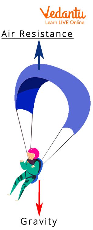
Terminal velocity is particularly relevant in applications such as skydiving, where the body or parachute reaches a steady descent rate.

Shape and Drag Coefficient

The shape of an object significantly influences its drag coefficient. Streamlined shapes reduce \(C_d\), thereby minimizing air resistance, while blunt or irregular shapes increase \(C_d\). Below are typical drag coefficients for various shapes:

Shape	Drag Coefficient (\(C_d\))
Sphere	~0.47
Cube	~1.05
Streamlined Car	~0.3 - 0.4
Flat Plate (perpendicular to flow)	~1.28
Teardrop	~0.04 - 0.1

These values are approximations and can vary based on specific design features and surface conditions.

Computational Fluid Dynamics (CFD) for Complex Cases

For objects with complex shapes or those moving at transonic and supersonic speeds, analytical formulas become insufficient for accurately predicting drag forces. In such cases, Computational Fluid Dynamics (CFD) simulations are employed. CFD allows for a detailed analysis of airflow patterns, compressibility effects, turbulence, and boundary layer behavior, providing precise drag force calculations tailored to specific conditions and geometries.

Viscous Drag and Surface Roughness

In addition to shape, the surface roughness of an object plays a vital role in determining the drag coefficient. Rough surfaces can induce earlier transition from laminar to turbulent flow, increasing the drag. Conversely, smooth surfaces can maintain laminar flow over larger portions of the object, reducing drag. This is particularly important in applications like aeronautical engineering, where minimizing drag is essential for fuel efficiency and performance.

Applications and Examples

1. Automotive Engineering

In automotive design, reducing air resistance is crucial for enhancing fuel efficiency and vehicle performance. Streamlined body shapes, smooth surfaces, and aerodynamic features like spoilers and air intakes are designed to minimize the drag coefficient, thereby reducing the overall drag force experienced by the vehicle.

2. Skydiving and Parachuting

Understanding terminal velocity is essential in skydiving and parachuting. The design of parachutes aims to increase the cross-sectional area (\(A\)) and optimize the drag coefficient (\(C_d\)) to ensure a safe and controlled descent. Variations in parachute shapes directly impact the terminal velocity achieved by the jumper.

3. Sports Equipment Design

Sports such as cycling, skiing, and swimming benefit from aerodynamic designs that reduce drag. Equipment like bicycle helmets, swimsuits, and ski suits are engineered to minimize air resistance, allowing athletes to achieve higher speeds with less effort.

4. Aerospace Engineering

Aerospace vehicles, including airplanes and rockets, require precise calculations of drag forces to ensure efficient propulsion and stability. The design of wings, fuselages, and other components is optimized to balance structural integrity with aerodynamic efficiency, reducing drag while maintaining performance.

Advanced Considerations

1. Compressibility Effects

At high velocities approaching and exceeding the speed of sound, air becomes compressible. Compressibility effects significantly alter the drag characteristics of objects, necessitating adjustments to the drag equations. Variable drag coefficients must be used to account for changes in air density and flow dynamics at these speeds.

2. Boundary Layer Effects

The boundary layer is the thin layer of air adjacent to the object's surface where viscous forces are significant. The behavior of the boundary layer—whether it is laminar or turbulent—affects the overall drag. Techniques such as boundary layer control and surface treatments are employed to manipulate the boundary layer, thereby influencing the drag coefficient.

3. Impact of Altitude

Air density (\(\rho\)) decreases with altitude, directly affecting the drag force experienced by objects. For applications like high-altitude flight or ballistic trajectories, variations in air density must be accounted for in drag calculations to ensure accurate performance predictions.

4. Temperature and Humidity

Temperature and humidity also influence air density and, consequently, the drag force. Higher temperatures can decrease air density, reducing drag, while increased humidity affects the viscosity of air, potentially altering flow characteristics and drag coefficients.

Summary

Air resistance is a fundamental force that plays a significant role in the motion of objects through the atmosphere. Accurately calculating drag force requires an understanding of various factors, including velocity, object shape, air density, and flow conditions. The basic drag equation serves as a starting point, with adjustments made based on the Reynolds number and flow regime to apply more specific formulas like Stokes' Law for laminar flow or the quadratic drag equation for turbulent flow.

For complex shapes and high-speed conditions, advanced computational methods such as CFD are indispensable for precise drag force predictions. Additionally, practical applications across automotive, aerospace, sports, and parachuting industries demonstrate the importance of aerodynamic considerations in optimizing performance and efficiency.

By comprehensively understanding and applying the appropriate air resistance formulas, engineers and scientists can design more efficient systems, enhance performance, and innovate in various technological domains.