Unlocking Data Secrets: Your Comprehensive Guide to Autoencoders

Key Insights into Autoencoders

Efficient Representation Learning: Autoencoders excel at learning compressed, meaningful representations of data in an unsupervised manner, primarily by reconstructing their input.
Versatile Architecture: They consist of an encoder (compressing data to a latent space) and a decoder (reconstructing data), with numerous variations like Denoising, Variational, and Convolutional AEs tailored for specific tasks.
Diverse Applications: Key uses include dimensionality reduction, anomaly detection, data denoising, feature extraction for other models, and even generative tasks like creating new data samples.

Decoding Autoencoders: The Fundamentals

Autoencoders represent a fascinating category of artificial neural networks primarily utilized for unsupervised learning. Their fundamental goal isn't necessarily prediction, like in many supervised learning tasks, but rather learning efficient representations (codings) of input data. Let's break down the core ideas.

What Exactly is an Autoencoder?

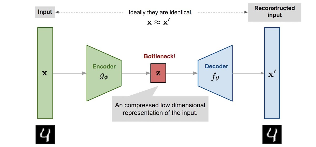
At its heart, an autoencoder is trained to perform a simple task: copy its input to its output. While this sounds trivial, the magic happens due to constraints imposed on the network architecture. By forcing the data through a compressed "bottleneck," the network must learn to capture the most salient features of the data to reconstruct it accurately. It learns an "identity function" approximately, focusing on encoding the input into a compressed form and then decoding it back.

The Core Components: Encoder, Bottleneck, and Decoder

Diagram comparing Autoencoder and Diffuser concepts

Conceptual overview comparing Autoencoders (focused on reconstruction via bottleneck) and Diffusers (focused on iterative denoising).

The Encoder

This part of the network takes the high-dimensional input data and maps (encodes) it into a lower-dimensional representation. It consists of one or more layers that progressively reduce the dimensionality.

The Bottleneck (Latent Space)

This is the crucial layer containing the compressed representation of the input. Its dimensionality is a key hyperparameter; if too small, it might lose important information (underfitting), and if too large (or equal to input), it might simply learn to copy without extracting meaningful features (overfitting), especially without regularization. This compressed representation is often called the "latent space" or "coding."

The Decoder

This part takes the compressed representation from the bottleneck layer and attempts to reconstruct (decode) the original high-dimensional input data. Its architecture often mirrors the encoder's but in reverse, using layers that increase dimensionality (e.g., transposed convolutions in image-based autoencoders).

Why Unsupervised Learning?

Autoencoders fall under unsupervised learning because they don't require labeled data for training. The input data itself provides the supervision signal: the network learns by comparing its reconstructed output to the original input and minimizing the difference (reconstruction error). This makes them powerful tools for exploring large, unlabeled datasets.

Training Dynamics and Architecture Nuances

Training an autoencoder involves optimizing the network's weights to minimize the reconstruction loss, forcing the encoder to learn useful compressions and the decoder to accurately reverse the process.

The Training Loop: Minimizing Reconstruction Loss

The core of training relies on backpropagation, just like other neural networks. The process involves:

Feeding input data through the encoder to obtain the latent representation.
Passing the latent representation through the decoder to get the reconstructed output.
Calculating a loss function that measures the dissimilarity between the original input and the reconstructed output.
Adjusting the weights of both the encoder and decoder via gradient descent to minimize this loss.

Choosing the Right Loss Function

The choice of loss function depends on the nature of the input data:

Mean Squared Error (MSE): Typically used for continuous, real-valued data (like pixel intensities in grayscale images). It measures the average squared difference between input and output values.
Binary Cross-Entropy (BCE): Suitable for binary data or data normalized to the range [0, 1] (like pixel values in MNIST digits). It measures the difference between probability distributions.

Using MSE can sometimes lead to blurry reconstructions in images, as it tends to average pixel values. More advanced loss functions (like perceptual loss) or integrating adversarial training can mitigate this.

Architectural Choices: Undercomplete vs. Overcomplete

Undercomplete Autoencoders

This is the classic setup where the bottleneck layer has a smaller dimension than the input layer. This constraint naturally forces the network to learn a compressed representation by capturing the principal variations in the data.

Overcomplete Autoencoders

Here, the bottleneck dimension is larger than or equal to the input dimension. Without constraints, these networks risk learning the identity function trivially (just copying input to output) without extracting useful features. To make them learn meaningful representations, regularization techniques (like sparsity) are essential.

A Spectrum of Autoencoders: Types and Variations

The basic autoencoder concept has been extended into various specialized architectures, each designed to impose different properties on the learned representation or handle specific data types.

Comparing Key Autoencoder Variants

Different autoencoder types offer unique strengths tailored to specific tasks. The following chart provides a comparative overview based on several key characteristics (Note: ratings are illustrative, based on typical performance and goals, on a scale where higher is generally better/more capable, with a minimum axis value for clarity).

Denoising Autoencoders (DAEs)

DAEs are trained to reconstruct the original, clean input from a corrupted version (e.g., adding Gaussian noise or masking parts of the input). This forces the model to learn more robust features that capture the underlying structure rather than superficial noise patterns.

Sparse Autoencoders

These introduce a sparsity constraint on the activations in the bottleneck layer. Typically, this is done by adding a penalty term to the loss function (e.g., L1 regularization or a KL divergence term) that encourages most neurons in the hidden layer to be inactive (output close to zero) for any given input. This promotes learning disentangled, meaningful features.

Variational Autoencoders (VAEs)

VAEs are a generative variant. Instead of mapping the input to a single fixed point in the latent space, the encoder outputs parameters (mean and variance) of a probability distribution (usually Gaussian). The decoder then samples from this distribution to generate the output. This probabilistic approach allows VAEs to generate new data samples similar to the training data by sampling points from the learned latent distribution. Training involves minimizing both reconstruction loss and a KL divergence term that keeps the learned distribution close to a standard Gaussian prior.

Convolutional Autoencoders (CAEs)

Specifically designed for grid-like data such as images, CAEs replace the fully connected layers of a standard autoencoder with convolutional layers in the encoder (for feature extraction and downsampling) and transposed convolutional layers (or upsampling + convolution) in the decoder (for reconstruction). This architecture respects the spatial hierarchy and locality of features in images.

Contractive Autoencoders (CAEs)

These add a penalty term to the loss function that encourages the learned representation to be robust to small perturbations in the input. Specifically, it penalizes the Jacobian (gradient) of the encoder's output with respect to the input, forcing the mapping to "contract" locally.

Quantum Autoencoders (QAEs)

An emerging area exploring the use of quantum computing principles. QAEs aim to leverage quantum circuits for encoding and decoding, potentially offering advantages for compressing and processing very high-dimensional quantum states or classical data encoded into quantum states, especially on future fault-tolerant quantum computers.

Putting Autoencoders to Work: Applications

The ability of autoencoders to learn meaningful representations from unlabeled data makes them valuable across a wide range of machine learning tasks.

Visualizing Autoencoder Applications

The mindmap below illustrates the diverse areas where autoencoders find practical use, stemming from their core capabilities in compression, reconstruction, and feature learning.

mindmap root["Autoencoders: Applications Landscape"] id1["Dimensionality Reduction"] id1.1["Data Visualization (e.g., t-SNE on latent space)"] id1.2["Preprocessing for other ML models"] id1.3["Comparison to PCA (Non-linear advantage)"] id2["Anomaly / Outlier Detection"] id2.1["Train on normal data"] id2.2["High reconstruction error indicates anomaly"] id2.3["Industrial defect detection"] id2.4["Fraud detection"] id3["Data Denoising & Restoration"] id3.1["Image denoising (DAEs)"] id3.2["Signal processing"] id3.3["Image reconstruction (e.g., MRI)"] id4["Feature Extraction / Learning"] id4.1["Learning meaningful features from raw data"] id4.2["Input for classification/clustering tasks"] id4.3["Transfer learning (using the encoder)"] id5["Generative Modeling (VAEs)"] id5.1["Image synthesis"] id5.2["Data augmentation"] id5.3["Drug discovery (molecule generation)"] id6["Other Areas"] id6.1["Natural Language Processing (NLP)
(e.g., learning word embeddings)"] id6.2["Facial Recognition (feature learning)"] id6.3["Recommender Systems (latent factor models)"]

Key Application Areas Explained

Dimensionality Reduction

Perhaps the most intuitive application. Autoencoders can compress high-dimensional data into a lower-dimensional latent space while preserving the most important information. Unlike Principal Component Analysis (PCA), which is limited to linear transformations, autoencoders can learn complex, non-linear mappings, often resulting in better representations for complex datasets.

Anomaly Detection

Autoencoders are effective anomaly detectors when trained primarily on "normal" data. The underlying assumption is that the autoencoder will learn to reconstruct normal patterns well (low reconstruction error) but will struggle to reconstruct anomalous data points that deviate significantly from the learned patterns (high reconstruction error). By setting a threshold on the reconstruction error, anomalies can be identified.

Data Denoising

As seen with Denoising Autoencoders (DAEs), these models can be explicitly trained to remove noise from data. By learning to map corrupted inputs back to their clean originals, they effectively learn the underlying data manifold and filter out noise.

Feature Extraction

The encoder part of a trained autoencoder can be used as a feature extractor. The learned latent representation often captures more salient and discriminative features than the raw input data. These compressed features can then be fed into other supervised learning models (like classifiers or regressors), potentially improving their performance, especially when labeled data is scarce (semi-supervised learning or pretraining).

Generative Modeling

Variational Autoencoders (VAEs) are powerful generative models. After training, new data samples can be generated by sampling points from the latent space distribution and passing them through the decoder network. This is widely used in image generation, music generation, and even drug discovery.

Practical Considerations and Advanced Concepts

Implementing and utilizing autoencoders effectively involves understanding certain nuances, best practices, and more advanced variations.

Key Characteristics of Autoencoder Types

The following table summarizes the core goals and characteristics of the most common autoencoder variants:

Autoencoder Type	Primary Goal	Typical Input	Latent Space Characteristic	Key Application(s)
Vanilla (Undercomplete)	Dimensionality Reduction, Feature Learning	General vectors	Compressed (Lower Dimension)	Dimensionality Reduction, Feature Extraction
Denoising	Robust Feature Learning, Noise Removal	Noisy Data	Learns to ignore noise	Image/Signal Denoising, Robust Features
Sparse	Meaningful Feature Learning, Disentanglement	General vectors	Sparsely Activated Neurons	Feature Extraction, Classification
Variational (VAE)	Generative Modeling, Probabilistic Encoding	General vectors	Represents a probability distribution	Data Generation, Image Synthesis
Convolutional	Spatial Hierarchy Learning (Images)	Images, Grids	Preserves Spatial Information	Image Compression, Denoising, Generation
Contractive	Robustness to Input Perturbations	General vectors	Low sensitivity to small input changes	Robust Feature Learning

Choosing Latent Space Dimensionality

Selecting the size of the bottleneck layer requires balancing compression and information retention. Too small, and the model might not capture enough detail for accurate reconstruction (underfitting). Too large, and it might learn trivial solutions or overfit, especially without regularization. This is often determined through experimentation and validation.

Regularization Techniques

Besides sparsity and contractive penalties, standard regularization techniques like L1/L2 weight decay and dropout can be applied to autoencoder layers to prevent overfitting and encourage learning more generalizable features.

Autoencoders vs. PCA

While both are used for dimensionality reduction, Principal Component Analysis (PCA) is restricted to finding a linear subspace that captures the maximum variance. Autoencoders, being neural networks, can learn complex, non-linear manifolds, potentially capturing the data structure more effectively than PCA for intricate datasets. However, PCA is computationally cheaper and deterministic.

Advanced Variants: Adversarial Autoencoders (AAEs)

AAEs combine ideas from VAEs and Generative Adversarial Networks (GANs). They use an adversarial training approach to force the aggregated posterior distribution of the latent space to match a chosen prior distribution (like a Gaussian), often leading to better generative quality than standard VAEs.

Autoencoders for Pretraining

The encoder learned by an autoencoder on a large unlabeled dataset can serve as an excellent weight initialization for a supervised model (like a classifier) trained on a smaller labeled dataset. This pretraining step helps the supervised model start with meaningful feature extractors, often leading to faster convergence and better performance.

Building and Evaluating Autoencoders

Frameworks like TensorFlow/Keras and PyTorch make building autoencoders relatively straightforward. Evaluating their performance, however, depends on the intended application.

Implementation Example (Conceptual)

Modern deep learning libraries provide high-level APIs to define the encoder and decoder networks. For instance, using Keras, one might define sequential models for the encoder and decoder with Dense layers (for vector data) or Conv2D/Conv2DTranspose layers (for images), connect them, and compile the combined autoencoder model with an appropriate optimizer (e.g., Adam) and loss function (e.g., MSE).

Watch: Building Your First Autoencoder

For a practical walkthrough, this video provides a guide on implementing a basic autoencoder using Keras, covering the essential steps from defining the architecture to training the model on a dataset like MNIST.

Evaluation Metrics

Performance evaluation depends on the goal:

Reconstruction Quality: Measured by the loss function value (MSE, BCE) on a test set. For images, metrics like Peak Signal-to-Noise Ratio (PSNR) or Structural Similarity Index Measure (SSIM) can provide more perceptual insights than raw MSE.
Dimensionality Reduction/Feature Extraction: Evaluate the quality of the latent representations by using them as input features for a downstream task (e.g., classification) and measuring that task's performance. Visualizing the latent space using techniques like t-SNE or UMAP can also provide qualitative insights.
Anomaly Detection: Assessed using standard classification metrics (Precision, Recall, F1-score, AUC) on a test set containing both normal and anomalous data points, based on a threshold applied to the reconstruction error.
Generative Quality (VAEs): Often evaluated qualitatively by inspecting generated samples, or quantitatively using metrics like Frechet Inception Distance (FID) or Inception Score (IS) for images.

Troubleshooting Common Issues

Blurry Reconstructions

Often occurs when using MSE loss for images. Consider using alternative loss functions (e.g., perceptual loss) or architectures incorporating adversarial components (like AAEs or VAE-GANs).

Model Not Converging / Poor Reconstruction

Check learning rate, network capacity (number of layers/neurons), activation functions, initialization (e.g., He/Xavier initialization), and ensure data is properly preprocessed/normalized.

Frequently Asked Questions (FAQ)

What's the main difference between an autoencoder and PCA?

Both are used for dimensionality reduction, but PCA (Principal Component Analysis) is a linear technique that finds orthogonal axes of maximum variance. Autoencoders are neural networks and can learn complex, non-linear relationships in the data. This makes autoencoders potentially more powerful for capturing intricate data structures, but they are computationally more expensive and lack the clear interpretability of PCA components.

Can autoencoders be used for classification?

Directly, a standard autoencoder is not a classifier as it's trained for reconstruction (unsupervised). However, they are often used *in conjunction* with classification. The encoder part can be used to extract meaningful features (latent representations) from the input data. These features can then be fed into a separate, typically simpler, classification model (like logistic regression, SVM, or a small neural network). This is particularly useful for pretraining or when dealing with high-dimensional data where raw input might not be optimal for classification.

What does "lossy" compression mean for autoencoders?

Lossy compression means that the reconstructed output is not perfectly identical to the original input; some information is lost during the compression (encoding) and decompression (decoding) process. This is inherent to most autoencoders, especially undercomplete ones, as the bottleneck forces the network to discard less important information to fit the data into a smaller representation. While the goal is to minimize this loss for relevant features, perfect reconstruction is rare and often not even desirable (as it might imply overfitting or simply copying). The "loss" refers to information loss, not the training loss function (though they are related).

How do Variational Autoencoders (VAEs) generate new data?

Unlike standard autoencoders that map input to a single point in latent space, a VAE's encoder maps input to the parameters (mean and variance) of a probability distribution (usually Gaussian) in the latent space. To generate new data after training, you don't need an input image. Instead, you randomly sample a point from the prior distribution (typically a standard Gaussian N(0,1)) defined over the latent space. This sampled point (a latent vector) is then fed into the trained decoder network, which transforms it back into the data space (e.g., generating a new image). Because the VAE learns a smooth, continuous latent space, points sampled from this space should decode into realistic-looking data samples similar to the training set.