Unveiling the Mysteries of Induced EMF: How Does a Changing Magnetic Field Generate Voltage?

Calculating the average voltage induced in a circular region by a time-varying magnetic field across two distinct phases.

Highlights

Faraday's Law Governs: The average induced electromotive force (EMF) is directly proportional to the rate of change of magnetic flux through the circular region.
Total Change Matters: To find the average EMF over the entire duration, we consider the magnetic flux at the very beginning (zero field) and the very end (downward field), divided by the total elapsed time.
Lenz's Law Determines Direction: The direction of the induced EMF (counterclockwise in this case) opposes the overall change in magnetic flux, ensuring energy conservation.

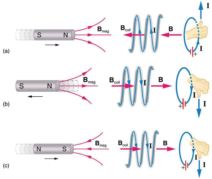
Diagram illustrating Lenz's Law with changing magnetic flux through a loop

Illustration of Lenz's Law: The induced current creates a magnetic field opposing the change in external flux.

Understanding Faraday's Law and Magnetic Flux

The phenomenon described in the query is a direct application of electromagnetic induction, primarily governed by Faraday's Law and Lenz's Law. When the magnetic field passing through a defined area changes over time, it induces an electromotive force (EMF), which is essentially a voltage, around the boundary of that area. This induced EMF can drive a current if a conductive path exists.

Faraday's Law Explained

Faraday's Law of Induction quantifies the induced EMF. It states that the magnitude of the induced EMF (\(\mathcal{E}\)) in any closed circuit is equal to the negative of the time rate of change of the magnetic flux (\(\Phi_B\)) through the circuit.

\[ \mathcal{E} = -N \frac{d\Phi_B}{dt} \]

Here, \(N\) is the number of turns in the loop (for the border of a single region, \(N=1\)). The derivative \( \frac{d\Phi_B}{dt} \) represents the instantaneous rate of change of magnetic flux. For calculating the average induced EMF over a time interval \(\Delta t\), we use the total change in flux \(\Delta \Phi_B\):

\[ \mathcal{E}_{avg} = -N \frac{\Delta \Phi_B}{\Delta t} \]

Defining Magnetic Flux

Magnetic flux (\(\Phi_B\)) is a measure of the total magnetic field lines passing through a given area. It depends on the strength of the magnetic field (\(B\)), the area (\(A\)), and the orientation between the field and the area.

Formula

For a uniform magnetic field perpendicular to a flat surface area \(A\), the magnetic flux is simplified. In general:

\[ \Phi_B = B A \cos\theta \]

Where:

\(B\) is the magnitude of the magnetic field.
\(A\) is the area of the surface.
\(\theta\) is the angle between the magnetic field direction and the vector normal (perpendicular) to the surface.

In this problem, the field is always perpendicular to the circular plane. If we define the normal vector as upward, then an upward field has \(\theta = 0^\circ\) (\(\cos 0^\circ = 1\)) and a downward field has \(\theta = 180^\circ\) (\(\cos 180^\circ = -1\)). Alternatively, we can assign a sign to B (+ for upward, - for downward) and keep \(\theta = 0^\circ\).

Units

The SI unit for magnetic flux is the Weber (Wb), where \(1 \, \text{Wb} = 1 \, \text{Tesla} \cdot \text{meter}^2 \, (\text{T} \cdot \text{m}^2)\).

Step-by-Step Calculation of Average Induced EMF

Let's apply these principles to calculate the average induced EMF over the entire duration described.

Defining the Problem Parameters

Radius of the circular region: \(r = 1.70 \, \text{mm} = 1.70 \times 10^{-3} \, \text{m}\)
Phase 1: \(B\) changes from \(B_0 = 0 \, \text{T}\) to \(B_1 = +1.50 \, \text{T}\) (upward) in \(\Delta t_1 = 150 \, \text{ms} = 0.150 \, \text{s}\)
Phase 2: \(B\) changes from \(B_1 = +1.50 \, \text{T}\) to \(B_2 = -0.500 \, \text{T}\) (downward) in \(\Delta t_2 = 85.0 \, \text{ms} = 0.0850 \, \text{s}\)
Target: Average EMF (\(\mathcal{E}_{avg}\)) over the total time \(\Delta t_{total} = \Delta t_1 + \Delta t_2\).
Number of turns: \(N=1\) (border of the region).

Calculating the Area

The area \(A\) of the circular region is:

\[ A = \pi r^2 = \pi (1.70 \times 10^{-3} \, \text{m})^2 \] \[ A = \pi (2.89 \times 10^{-6} \, \text{m}^2) \approx 9.0792 \times 10^{-6} \, \text{m}^2 \]

Determining Initial and Final Magnetic Flux over the Total Period

We need the flux at the very beginning of the process (\(t=0\)) and at the very end (\(t = \Delta t_1 + \Delta t_2\)). We assign positive to upward field/flux and negative to downward field/flux.

Initial Flux (\(\Phi_{initial}\) at \(t=0\)): \[ \Phi_{initial} = B_0 \cdot A = (0 \, \text{T}) \cdot A = 0 \, \text{Wb} \]
Final Flux (\(\Phi_{final}\) at \(t = 150 \, \text{ms} + 85.0 \, \text{ms} = 235 \, \text{ms}\)): The final field is \(B_2 = -0.500 \, \text{T}\) (downward). \[ \Phi_{final} = B_2 \cdot A = (-0.500 \, \text{T}) \times (9.0792 \times 10^{-6} \, \text{m}^2) \] \[ \Phi_{final} \approx -4.5396 \times 10^{-6} \, \text{Wb} \]
Total Change in Flux (\(\Delta \Phi_{total}\)): \[ \Delta \Phi_{total} = \Phi_{final} - \Phi_{initial} \] \[ \Delta \Phi_{total} = (-4.5396 \times 10^{-6} \, \text{Wb}) - (0 \, \text{Wb}) \] \[ \Delta \Phi_{total} \approx -4.5396 \times 10^{-6} \, \text{Wb} \]

Calculating the Total Time Interval

The average EMF is calculated over the entire duration:

\[ \Delta t_{total} = \Delta t_1 + \Delta t_2 = 150 \, \text{ms} + 85.0 \, \text{ms} = 235 \, \text{ms} \] \[ \Delta t_{total} = 0.235 \, \text{s} \]

Applying Faraday's Law for Average EMF

Now we use Faraday's Law for the average EMF with \(N=1\):

\[ \mathcal{E}_{avg} = -N \frac{\Delta \Phi_{total}}{\Delta t_{total}} = -1 \times \frac{-4.5396 \times 10^{-6} \, \text{Wb}}{0.235 \, \text{s}} \] \[ \mathcal{E}_{avg} = \frac{4.5396 \times 10^{-6}}{0.235} \, \text{V} \] \[ \mathcal{E}_{avg} \approx 1.9317 \times 10^{-5} \, \text{V} \]

The question asks for the magnitude in microvolts (\(\mu V\)). We convert Volts to microvolts (\(1 \, \text{V} = 10^6 \, \mu V\)):

\[ \mathcal{E}_{avg} \approx (1.9317 \times 10^{-5}) \times 10^6 \, \mu\text{V} \] \[ \mathcal{E}_{avg} \approx 19.317 \, \mu\text{V} \]

Rounding to three significant figures, based on the precision of the given values:

Magnitude of Average Induced EMF = 19.3 µV

Determining the Direction using Lenz's Law

Lenz's Law Explained

Lenz's Law provides the direction of the induced EMF and any resulting induced current. It's essentially a consequence of the conservation of energy applied to electromagnetic induction. The law states that the direction of the induced current (and thus the polarity of the induced EMF) is such that it creates a magnetic field that opposes the change in magnetic flux that produced it.

Applying Lenz's Law to this Scenario

Identify the Change in Flux (\(\Delta \Phi_{total}\)): Over the total time period (0 to 235 ms), the magnetic flux changed from 0 Wb to approximately \(-4.54 \times 10^{-6}\) Wb. This represents a net increase in downward flux (or a change towards more negative flux).
Determine the Direction of the Opposing Field: To oppose this increase in downward flux, the induced current must generate its own magnetic field directed upward.
Use the Right-Hand Rule: To find the direction of current that produces an upward magnetic field through the circular loop, curl the fingers of your right hand in the direction of the current. Your thumb will point in the direction of the induced magnetic field. For the induced field to point upward (out of the page when viewed from above), your fingers must curl in a counterclockwise direction.

Therefore, the direction of the average induced EMF (and the induced current, if a path exists) around the border of the circular region, as seen from above, is counterclockwise.

Summary Table: Magnetic Field and Flux Changes

This table summarizes the state of the magnetic field and the resulting magnetic flux through the circular area at key points in time.

Time Point	Elapsed Time (ms)	Magnetic Field (B)	Direction	Magnetic Flux (\(\Phi_B\), Wb)
Initial	0	0 T	N/A	0
End of Phase 1	150	1.50 T	Upward	\(+1.50 \times A \approx +1.36 \times 10^{-5}\)
End of Phase 2 (Final)	235	0.500 T	Downward	\(-0.500 \times A \approx -4.54 \times 10^{-6}\)

Note: \(A \approx 9.0792 \times 10^{-6} \, \text{m}^2\). Positive flux corresponds to upward field, negative flux to downward field.

Visualizing Magnetic Field and Flux Changes

Radar Chart: Comparing Key Parameters Across Phases

This radar chart visualizes the relative magnitudes of key parameters during each phase and over the total duration. The values are scaled relative to the maximum observed value for each parameter across the phases (approximate maximums used: Δt=250ms, |ΔB|=2.0T, |ΔΦ|=20000nWb, |Avg EMF|=250μV) and plotted on a scale from 0.5 to 10 for better visibility.

The chart highlights that Phase 2 involves the largest change in magnetic field magnitude (from +1.5 T to -0.5 T, a change of 2.0 T) and the largest change in flux over its shorter duration, leading to the highest average EMF during that interval. However, the overall average EMF considers the net change from start to finish over the total time, resulting in a smaller value.

Mindmap: Concepts of Electromagnetic Induction

This mindmap illustrates the key concepts involved in understanding and solving this electromagnetic induction problem.

mindmap root["Electromagnetic Induction"] id1["Faraday's Law"] id1a["Induced EMF (\(\mathcal{E}\))"] id1a1["Proportional to rate
of change of Flux"] id1a2["Formula: \(\mathcal{E} = -N \frac{d\Phi_B}{dt}\)"] id1b["Average EMF"] id1b1["Formula: \(\mathcal{E}_{avg} = -N \frac{\Delta\Phi_B}{\Delta t}\)"] id2["Magnetic Flux (\(\Phi_B\))"] id2a["Definition"] id2a1["Measure of magnetic field
lines through an area"] id2a2["Formula: \(\Phi_B = B A \cos\theta\)"] id2b["Factors Affecting Flux"] id2b1["Magnetic Field Strength (B)"] id2b2["Area (A)"] id2b3["Angle (\(\theta\))"] id2c["Units: Weber (Wb)"] id3["Lenz's Law"] id3a["Direction of Induced EMF/Current"] id3a1["Opposes the change
in magnetic flux"] id3b["Based on Conservation of Energy"] id3c["Use Right-Hand Rule"] id4["This Specific Problem"] id4a["Changing Magnetic Field (B)"] id4a1["Phase 1: 0 to +1.5T"] id4a2["Phase 2: +1.5T to -0.5T"] id4a3["Overall: 0 to -0.5T"] id4b["Circular Region"] id4b1["Fixed Area (A)"] id4b2["Fixed Angle (\(\theta=0^\circ\) or \(180^\circ\))"] id4c["Calculate Average EMF
over Total Time (\(\Delta t_{total}\))"]

Deeper Dive: Induced EMF in Action

To further understand Faraday's Law and the concept of average induced EMF, this video provides explanations and examples related to calculating EMF from changing magnetic flux, similar to the principles used here.

Video explaining Faraday's Law and the calculation of average EMF.

The video discusses how changes in magnetic flux lead to induced EMF, covering the core formula \(\mathcal{E} = -\Delta\Phi / \Delta t\). It reinforces the concepts applied in calculating the average EMF over the specified time interval in this problem, connecting the theoretical laws to practical calculations.

References

Last updated May 1, 2025