Unveiling the Secrets of Induced EMF: How a Changing Magnetic Field Creates Voltage

When a magnetic field passing through a loop or region changes over time, it induces an electromotive force (emf), which can drive an electric current. This phenomenon, known as electromagnetic induction, is governed by Faraday's Law and Lenz's Law. Let's delve into calculating the average induced emf for the specific scenario described.

Key Insights

Faraday's Law Quantifies Induction: The magnitude of the induced emf is directly proportional to the rate at which the magnetic flux through the circuit changes.
Lenz's Law Determines Direction: The induced emf (and any resulting current) always acts in a direction that opposes the change in magnetic flux that produced it.
Calculation Requires Specifics: To find the numerical value of the induced emf, we need the initial and final magnetic field strengths, the area of the region, and the time interval over which the change occurs.

Understanding Electromagnetic Induction

Electromagnetic induction is a fundamental principle in physics, describing how a changing magnetic environment can produce an electric voltage (emf) in a conductor. Two key laws govern this process:

Faraday's Law of Induction

Faraday's Law states that the average induced emf (\(\mathcal{E}_{avg}\)) in any closed loop is proportional to the rate of change of the magnetic flux (\(\Phi\)) through the loop. Mathematically, for a single loop (N=1):

\[ \mathcal{E}_{avg} = - \frac{\Delta \Phi}{\Delta t} \] Where:

\(\Delta \Phi\) is the change in magnetic flux.
\(\Delta t\) is the time interval over which the change occurs.
The negative sign indicates the direction of the induced emf, as specified by Lenz's Law.

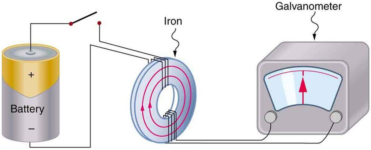
Magnetic flux (\(\Phi\)) itself is a measure of the total magnetic field lines passing through a given area. For a uniform magnetic field \(B\) perpendicular to a flat area \(A\), the flux is simply: \[ \Phi = B \cdot A \] If the field makes an angle \(\theta\) with the normal (perpendicular) to the area, the formula becomes \(\Phi = B A \cos \theta\). Diagram illustrating magnetic flux through a loop

Diagram illustrating magnetic flux through a loop

Illustration of magnetic flux lines passing through a surface area.

Lenz's Law

Lenz's Law provides the direction of the induced emf and current. It states that the direction is always such that the magnetic field created by the induced current opposes the change in the original magnetic flux.

If the magnetic flux through a loop increases, the induced current creates a magnetic field in the opposite direction to the original field.
If the magnetic flux decreases, the induced current creates a magnetic field in the same direction as the original field, attempting to maintain the flux.

Diagram showing Lenz's Law: the induced current opposes the change in flux.

Calculating the Average Induced EMF

We are asked to find the average induced emf around the border of a flat, horizontal circular region during an 85.0 ms interval where the magnetic field changes to 0.500 T pointing downward.

Step 1: Define Parameters and Assumptions

Based on context from similar problems often encountered in physics exercises (as referenced in the provided materials), we'll assume the following parameters:

Radius of the circular region (r): 170 mm = 0.170 m
Initial Magnetic Field (\(B_i\)): 0.125 T, pointing upward. We define the upward direction as positive. So, \(B_i = +0.125 \, \text{T}\).
Final Magnetic Field (\(B_f\)): 0.500 T, pointing downward. So, \(B_f = -0.500 \, \text{T}\).
Time Interval (\(\Delta t\)): 85.0 ms = \(85.0 \times 10^{-3} \, \text{s} = 0.0850 \, \text{s}\).
Orientation: The magnetic field is perpendicular to the horizontal circular region. The angle \(\theta\) between the field direction and the area normal (chosen as upward) is either 0° or 180°. The flux is \(\Phi = B A\), where B can be positive (upward) or negative (downward).

Step 2: Calculate the Area

The area \(A\) of the circular region is given by:

\[ A = \pi r^2 = \pi (0.170 \, \text{m})^2 = \pi (0.0289 \, \text{m}^2) \approx 0.090792 \, \text{m}^2 \]

Step 3: Calculate the Change in Magnetic Flux (\(\Delta \Phi\))

The change in magnetic flux is the difference between the final and initial flux. Since the area is constant and the field is perpendicular:

\[ \Delta \Phi = \Phi_f - \Phi_i = (B_f \cdot A) - (B_i \cdot A) = (B_f - B_i) \cdot A \] First, find the change in the magnetic field strength: \[ \Delta B = B_f - B_i = (-0.500 \, \text{T}) - (+0.125 \, \text{T}) = -0.625 \, \text{T} \] Now, calculate the change in flux: \[ \Delta \Phi = (\Delta B) \cdot A = (-0.625 \, \text{T}) \cdot (0.090792 \, \text{m}^2) \approx -0.056745 \, \text{Wb} \] The unit of magnetic flux is the Weber (Wb), where \(1 \, \text{Wb} = 1 \, \text{T} \cdot \text{m}^2\).

Step 4: Calculate the Magnitude of the Average Induced EMF

Using Faraday's Law, the magnitude of the average induced emf is:

\[ |\mathcal{E}_{avg}| = \left| - \frac{\Delta \Phi}{\Delta t} \right| = \frac{|\Delta \Phi|}{\Delta t} \] \[ |\mathcal{E}_{avg}| = \frac{|-0.056745 \, \text{Wb}|}{0.0850 \, \text{s}} \approx \frac{0.056745}{0.0850} \, \text{V} \approx 0.66759 \, \text{V} \] The unit of emf is the Volt (V), where \(1 \, \text{V} = 1 \, \text{Wb} / \text{s}\).

Step 5: Convert to Microvolts (µV)

The question asks for the magnitude in microvolts (µV). We convert Volts to microvolts by multiplying by \(10^6\):

\[ |\mathcal{E}_{avg}| \approx 0.66759 \, \text{V} \times 10^6 \, \frac{\mu\text{V}}{\text{V}} \approx 667,590 \, \mu\text{V} \] Rounding to three significant figures (consistent with the input data): \[ |\mathcal{E}_{avg}| \approx 668,000 \, \mu\text{V} \] Or, \(6.68 \times 10^5 \, \mu\text{V}\).

Step 6: Determine the Direction of the Induced EMF

We apply Lenz's Law. The magnetic field changes from upward (+0.125 T) to downward (-0.500 T). The net change in flux (\(\Delta \Phi\)) is negative (downward flux increased or upward flux decreased significantly). The induced emf must create a magnetic field that opposes this change.

The change is towards a stronger downward field (or less upward field).
To oppose this change, the induced magnetic field must point upward.

Using the right-hand rule for a loop viewed from above:

Curl the fingers of your right hand in the direction of the current flow around the loop.
Your thumb points in the direction of the magnetic field produced by that current.

To produce an upward induced magnetic field, the induced current (and thus the emf) must flow in a counterclockwise direction when viewed from above.

The right-hand rule helps determine the direction of the magnetic field produced by a current loop. An upward field requires a counterclockwise current from above.

Summary of Results

Magnitude: 668,000 µV
Direction (as seen from above): Counterclockwise

Visualizing the Factors Affecting Induced EMF

The magnitude of the induced EMF depends on several factors. The radar chart below provides a conceptual comparison of how different parameters influence the induced EMF, based on Faraday's Law (\(\mathcal{E} = -N \frac{\Delta(BA\cos\theta)}{\Delta t}\)). We compare our scenario (high rate of change, moderate area, perpendicular field, single turn) to hypothetical variations.

This chart illustrates that the rate of change of the magnetic field, the alignment of the field with the area normal, the area itself, and the number of turns in a coil are all crucial factors. In our specific problem, the significant change in B over a short time (\(\Delta B / \Delta t\)) is the primary driver for the large induced emf, even with a single loop (N=1).

Conceptual Map of Electromagnetic Induction

The mind map below illustrates the interconnected concepts involved in calculating the induced emf, starting from the changing magnetic field and leading to the final result through Faraday's and Lenz's laws.

mindmap root["Electromagnetic Induction"] id1["Changing Magnetic Field (ΔB/Δt)"] id1a["Source of Induction"] id2["Magnetic Flux (Φ)"] id2a["Φ = B ⋅ A ⋅ cos θ"] id2b["Depends on:"] id2b1["Field Strength (B)"] id2b2["Area (A)"] id2b3["Orientation (θ)"] id3["Change in Magnetic Flux (ΔΦ)"] id3a["ΔΦ = Φ_final - Φ_initial"] id4["Faraday's Law"] id4a["Relates ΔΦ/Δt to EMF"] id4b["Formula: E = -N (ΔΦ / Δt)"] id4b1["Magnitude of EMF"] id4b2["Number of Turns (N)"] id4b3["Rate of Flux Change"] id5["Lenz's Law"] id5a["Determines Direction"] id5b["Induced Field Opposes ΔΦ"] id5b1["Direction of Induced EMF"] id5b2["Direction of Induced Current (if circuit exists)"] id6["Induced EMF (E)"] id6a["Calculated Magnitude (Volts or µV)"] id6b["Determined Direction (e.g., Clockwise/Counterclockwise)"]

This map highlights how a change in the magnetic field leads to a change in flux, which, according to Faraday's Law, induces an emf. Lenz's Law then dictates the direction of this induced emf.

Calculation Summary Table

This table summarizes the key parameters used and the results obtained in the calculation:

Parameter	Symbol	Value	Units
Radius	\(r\)	0.170	m
Area	\(A\)	\(\approx 0.090792\)	m²
Initial Magnetic Field	\(B_i\)	+0.125	T
Final Magnetic Field	\(B_f\)	-0.500	T
Change in Magnetic Field	\(\Delta B\)	-0.625	T
Time Interval	\(\Delta t\)	0.0850	s
Change in Magnetic Flux	\(\Delta \Phi\)	\(\approx -0.056745\)	Wb
Average Induced EMF (Magnitude)	\(\|\mathcal{E}_{avg}\|\)	\(\approx 0.668\)	V
Average Induced EMF (Magnitude)	\(\|\mathcal{E}_{avg}\|\)	668,000	µV
Direction (from above)	-	Counterclockwise	-

Further Exploration: Faraday's Law Explained

For a deeper conceptual understanding of Faraday's Law and the calculation of average induced emf, the following video provides a helpful explanation:

Video explaining Faraday's Law and average emf calculations.

This video discusses the relationship between changing magnetic flux and the resulting induced voltage, reinforcing the principles used in our calculation.

References

Last updated May 1, 2025