Unveiling the Electric Surge: How a Changing Magnetic Field Creates Voltage

When a magnetic field passing through a conductive loop or region changes, it doesn't just change silently – it generates an electrical effect! This phenomenon, known as electromagnetic induction, is fundamental to how generators, transformers, and many other technologies work. Your query describes exactly such a scenario: a magnetic field within a circular region changes its strength and direction over a short time. Let's delve into how to determine the resulting average induced electromotive force (EMF), which is essentially the average voltage generated around the border of this region.

Highlights: Key Insights into Induced EMF

Core Principles and Calculation Factors

Faraday's Law Governs: The magnitude of the induced EMF is directly proportional to how quickly the magnetic flux through the region changes. Faster change means higher voltage.
Lenz's Law Dictates Direction: The induced EMF (and any resulting current) will always create its own magnetic field that opposes the *change* in the original magnetic flux.
Crucial Missing Details: To calculate a precise numerical value for the EMF magnitude, the area of the circular region and the initial state (magnitude and direction) of the magnetic field before the change began are required.

Understanding the Foundation: Faraday's Law and Magnetic Flux

The Physics Behind Induced Voltage

The heart of this phenomenon lies in Faraday's Law of Induction. This law states that the induced electromotive force ($\varepsilon$) in any closed circuit is equal to the negative of the time rate of change of the magnetic flux ($\Phi$) enclosed by the circuit.

What is Magnetic Flux?

Magnetic flux ($\Phi$) is a measure of the total magnetic field lines passing through a given area. Imagine it as the "amount" of magnetism flowing through a surface. It depends on three factors:

Magnetic Field Strength (B): The stronger the magnetic field, the greater the flux. Measured in Teslas (T).
Area (A): The larger the area the field passes through, the greater the flux. Measured in square meters (m²).
Orientation ($\theta$): The angle between the magnetic field lines and the normal (a line perpendicular) to the surface area. Flux is maximum when the field is perpendicular to the surface ($\theta = 0^\circ$) and zero when parallel ($\theta = 90^\circ$).

The formula for magnetic flux is:

\[ \Phi = B A \cos\theta \]

A change in *any* of these factors (B, A, or $\theta$) over time will result in a change in magnetic flux, $\Delta\Phi$.

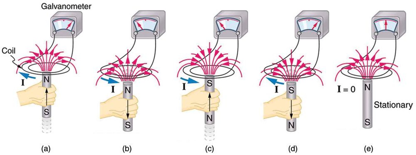
Diagram illustrating magnetic flux through a loop

Illustration of magnetic flux ($\Phi$) through a surface area (A) due to a magnetic field (B).

Calculating Average Induced EMF

Faraday's Law, when considering an average EMF over a specific time interval ($\Delta t$), is often written as:

\[ \varepsilon_{avg} = - \frac{\Delta\Phi}{\Delta t} = - \frac{\Phi_f - \Phi_i}{\Delta t} \] Where:

$\varepsilon_{avg}$ is the average induced EMF (in Volts, V).
$\Delta\Phi = \Phi_f - \Phi_i$ is the change in magnetic flux (final flux minus initial flux, in Webers, Wb).
$\Delta t$ is the time interval over which the flux changes (in seconds, s).

The negative sign is crucial and is related to Lenz's Law, which determines the direction of the induced EMF.

Addressing the Specifics: Calculation and Missing Information

Why Initial Conditions and Area Matter

Your query provides the final state of the magnetic field ($B_f = 0.500$ T, downward) and the time interval ($\Delta t = 85.0 \text{ ms} = 0.085 \text{ s}$). However, to calculate $\Delta\Phi = \Phi_f - \Phi_i$, we absolutely need:

The Initial Magnetic Flux ($\Phi_i$): This requires knowing the initial magnetic field magnitude ($B_i$) and its direction relative to the circular region (which determines $\theta_i$). Was the field initially zero? Pointing upward? Pointing downward but with a different strength? Each scenario leads to a different $\Delta\Phi$.
The Area of the Circular Region (A): The flux is proportional to the area ($A = \pi r^2$). Without the radius ($r$) or the area ($A$), we cannot calculate the flux values.

Without these pieces of information, we cannot provide a definitive numerical magnitude for the average induced EMF.

An Illustrative Calculation: Making Reasonable Assumptions

To demonstrate the calculation process, let's make some common assumptions often implied in such physics problems:

Assumption 1: Initial Field was Zero. Let's assume the magnetic field started at $B_i = 0$ T.
Assumption 2: Standard Loop Size. Let's assume the circular region has a radius of $r = 10.0 \text{ cm} = 0.100 \text{ m}$.

With these assumptions, we can proceed:

Step 1: Calculate the Area

\[ A = \pi r^2 = \pi (0.100 \text{ m})^2 = 0.0100\pi \text{ m}^2 \approx 0.0314 \text{ m}^2 \]

Step 2: Define the Normal and Calculate Fluxes

Let's define the normal vector to the circular area as pointing upward.

Initial Flux ($\Phi_i$): Since $B_i = 0$, $\Phi_i = 0$.
Final Flux ($\Phi_f$): The final field $B_f = 0.500$ T points downward. The angle between the downward field and the upward normal is $\theta_f = 180^\circ$. \[ \Phi_f = B_f A \cos(180^\circ) = (0.500 \text{ T}) (0.0100\pi \text{ m}^2) (-1) = -0.00500\pi \text{ Wb} \] \[ \Phi_f \approx -0.0157 \text{ Wb} \]

Step 3: Calculate the Change in Flux

\[ \Delta\Phi = \Phi_f - \Phi_i = -0.00500\pi \text{ Wb} - 0 = -0.00500\pi \text{ Wb} \] \[ \Delta\Phi \approx -0.0157 \text{ Wb} \]

Step 4: Calculate the Average Induced EMF Magnitude

\[ \varepsilon_{avg} = - \frac{\Delta\Phi}{\Delta t} = - \frac{-0.00500\pi \text{ Wb}}{0.085 \text{ s}} = \frac{0.00500\pi}{0.085} \text{ V} \] \[ \varepsilon_{avg} \approx 0.1848 \text{ V} \]

Step 5: Convert to Microvolts (µV)

The question asks for the magnitude in µV. Since $1 \text{ V} = 10^6 \text{ µV}$: \[ \varepsilon_{avg} \approx 0.1848 \times 10^6 \text{ µV} = 184,800 \text{ µV} \]

Important Note: This value of 184,800 µV is based entirely on the assumptions made (initial field = 0 T, radius = 10 cm). Different initial conditions or a different area would yield a different magnitude.

Determining the Direction: Lenz's Law in Action

Opposing the Change

Lenz's Law gives us the direction of the induced EMF (and the resulting current if the border is conductive). It states that the direction is always such that the magnetic field created by the induced current opposes the *change* in the original magnetic flux.

Let's apply this to our assumed scenario ($B_i = 0$, $B_f = 0.500$ T downward):

Identify the Change: The magnetic flux changed from zero to a value corresponding to a downward-pointing field. This is an *increase* in downward magnetic flux through the loop.
Oppose the Change: To oppose this *increase* in *downward* flux, the induced current must generate its own magnetic field that points *upward*.
Apply the Right-Hand Rule: To determine the current direction that produces an upward magnetic field inside the loop, use the right-hand rule for loops. Curl the fingers of your right hand in the direction of the current; your thumb points in the direction of the induced magnetic field inside the loop. For an *upward* field (thumb pointing up), your fingers must curl in a **counterclockwise** direction when viewed from above.

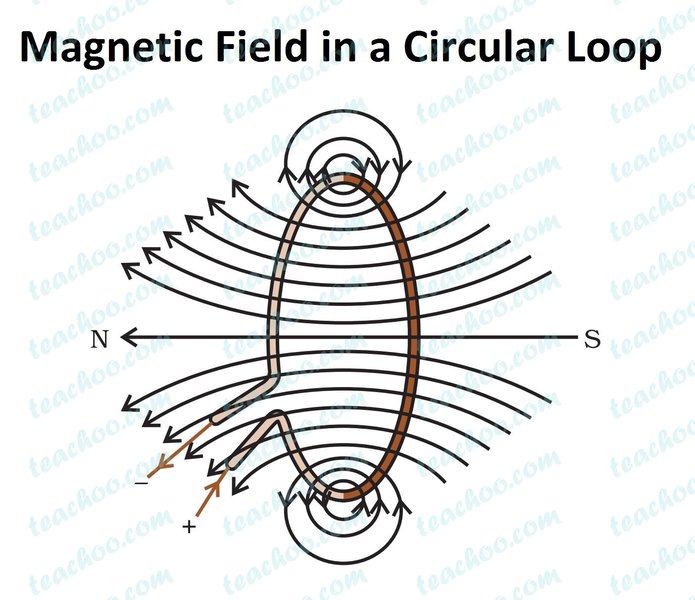
The Right-Hand Rule helps determine the direction of the magnetic field produced by a current loop. A counterclockwise current (viewed from above) creates an upward magnetic field inside the loop.

Therefore, based on the assumption that the magnetic field increased from zero to 0.500 T downward, the direction of the average induced EMF around the border is **counterclockwise** as seen from above.

What if the Initial Field Was Different?

If the initial field was, for example, 1.10 T downward, then the change would be from 1.10 T downward to 0.500 T downward. This is a *decrease* in downward flux. To oppose this decrease, the induced field would need to point *downward* (to reinforce the weakening field). According to the right-hand rule, a downward induced field requires a **clockwise** induced EMF/current. This highlights how critical the initial conditions are for determining both magnitude and direction.

Visualizing the Factors Influencing Induced EMF

Comparing Key Parameters

The magnitude of the induced EMF depends on several factors derived from Faraday's Law. The chart below provides a conceptual comparison of the relative importance or contribution of these factors to inducing a voltage. A higher score indicates a greater potential contribution to the EMF magnitude (assuming other factors are constant).

This radar chart illustrates that factors like the rate of change of the magnetic field, the area of the loop, and the number of turns (if it were a coil) generally have the most direct and significant impact on the induced EMF magnitude. The time interval inversely affects the *average* EMF (a shorter time for the same flux change leads to a higher average EMF). The initial magnetic field's magnitude is important primarily because it determines the *change* in the field ($\Delta B = B_f - B_i$).

Mapping the Concepts: Electromagnetic Induction

Connecting the Principles

The process of inducing an EMF involves several interconnected physics principles. This mindmap visualizes the relationship between the changing magnetic field, magnetic flux, Faraday's Law, Lenz's Law, and the resulting induced EMF.

mindmap root["Electromagnetic Induction"] id1["Magnetic Field (B)"] id1a["Changes Over Time (ΔB/Δt)"] id1b["Spatial Area (A)"] id1c["Orientation (cos θ)"] id2["Magnetic Flux (Φ = BAcosθ)"] id2a["Initial Flux (Φi)"] id2b["Final Flux (Φf)"] id2c["Change in Flux (ΔΦ = Φf - Φi)"] id3["Time Interval (Δt)"] id4["Faraday's Law
ε = -ΔΦ/Δt"] id4a["Magnitude of EMF
|ε| = |ΔΦ/Δt|"] id4a1["Depends on ΔB, A, Δt, Δcosθ"] id5["Lenz's Law
(Determines Direction)"] id5a["Induced Field Opposes ΔΦ"] id5a1["Use Right-Hand Rule"] id5a2["Direction (Clockwise/Counterclockwise)"] id6["Induced EMF (ε)"] id6a["Magnitude (Volts or µV)"] id6b["Direction"]

This mindmap shows how a changing magnetic field leads to a change in magnetic flux over a certain time. Faraday's Law quantitatively relates this change in flux over time to the magnitude of the induced EMF, while Lenz's Law provides the rule for determining the direction of that EMF by requiring opposition to the flux change.

Summarizing Potential Outcomes

Induced EMF Magnitude and Direction for Different Initial Fields

Since the initial magnetic field ($B_i$) significantly affects the result, the following table summarizes the expected outcome for the direction of the induced EMF based on different possible initial conditions, assuming the final field is $B_f = 0.500$ T downward and the normal to the area points upward.

Initial Magnetic Field ($B_i$)	Change in Downward Flux ($\Delta\Phi_{down}$)	Direction of Induced B-Field (Opposes Change)	Direction of Induced EMF (Viewed from Above)	EMF Magnitude $\|\varepsilon_{avg}\|$
0 T	Increase ($\Phi$ goes from 0 to negative)	Upward	Counterclockwise	$\propto A \|B_f\| / \Delta t$
0.200 T Upward	Increase ($\Phi$ goes from positive to negative)	Upward	Counterclockwise	$\propto A \|B_f + B_i\| / \Delta t$
0.200 T Downward	Increase ($\Phi$ goes from small negative to larger negative)	Upward	Counterclockwise	$\propto A \|B_f - B_i\| / \Delta t$
1.10 T Downward	Decrease ($\Phi$ goes from large negative to smaller negative)	Downward	Clockwise	$\propto A \|B_f - B_i\| / \Delta t$

This table clearly illustrates how the initial state dictates the direction of the induced EMF. An increase in downward flux always leads to a counterclockwise EMF, while a decrease leads to a clockwise EMF (when viewed from above).

Visualizing Induction Principles

Calculating Induced EMF Example

Many physics examples involve calculating induced EMF in loops due to changing magnetic fields. The video below provides a worked example demonstrating the application of Faraday's Law, similar to the principles discussed here.

Example problem solving for induced EMF using Faraday's Law.

This video walks through calculating the average induced EMF in a circular loop when the magnetic field changes uniformly over time. It reinforces the steps involving calculating the change in flux ($\Delta \Phi = \Delta B \times A$) and dividing by the time interval ($\Delta t$) to find the EMF magnitude, applying the core concepts of Faraday's Law.

References

Sources Used for This Analysis
Last updated May 1, 2025