Unlocking the Secrets of Cost Minimization: When Average Variable Cost Meets Marginal Cost

Key Highlights

Understanding Average Variable Cost (AVC): AVC represents the variable costs per unit of output, crucial for short-term production decisions.
Grasping Marginal Cost (MC): MC is the additional cost incurred by producing one more unit, essential for optimizing production levels.
The Intersection Point: AVC and MC intersect at the minimum point of the AVC curve, a pivotal point for cost-effective production.

Decoding Average Variable Cost (AVC) and Marginal Cost (MC)

In the realm of microeconomics, understanding the interplay between Average Variable Cost (AVC) and Marginal Cost (MC) is crucial for businesses aiming to optimize production and minimize expenses. AVC represents the variable costs (such as labor and materials) per unit of output. MC, on the other hand, signifies the additional cost incurred when producing one more unit of a good or service. Their relationship is visually represented by cost curves, where the marginal cost curve intersects the average variable cost curve at its lowest point.

Defining Average Variable Cost (AVC)

Average Variable Cost (AVC) is a key metric in economics that measures a firm's variable costs per unit of output. Variable costs are those expenses that fluctuate with the level of production, such as raw materials, direct labor, and energy. The formula for calculating AVC is:

\[ \text{AVC} = \frac{\text{Total Variable Costs (TVC)}}{\text{Quantity of Output (Q)}} \]

AVC is crucial for making short-term production decisions. It helps firms determine whether to continue production or temporarily shut down if the price falls below the AVC. For instance, if a Ugandan company producing textiles finds that its AVC per shirt is UGX 5,000, it needs to ensure that the selling price covers at least this amount to justify continued production.

Defining Marginal Cost (MC)

Marginal Cost (MC) is the change in total cost that arises when the quantity produced is incremented by one unit. It essentially reflects the cost of producing one additional unit of a product. The formula for calculating MC is:

\[ \text{MC} = \frac{\Delta \text{Total Cost (TC)}}{\Delta \text{Quantity of Output (Q)}} \]

Since fixed costs do not change with the level of production, MC is influenced solely by variable costs. Understanding MC is vital for optimizing production levels and maximizing profits. For example, a coffee farmer in Uganda might analyze the marginal cost of harvesting an additional kilogram of coffee beans to determine the most profitable production quantity. If the marginal cost exceeds the marginal revenue (the additional revenue from selling one more unit), the company is losing money on each additional unit produced.

The Interplay Between AVC and MC: The U-Shaped Curve

Both AVC and MC curves typically exhibit a U-shape. Initially, as production increases, both AVC and MC decrease due to economies of scale and increased efficiency. However, beyond a certain point, diminishing returns set in, leading to rising AVC and MC. This is because additional inputs become less productive, and costs increase at an increasing rate.

The marginal cost curve intersects the average variable cost curve at its minimum point. This intersection is not coincidental. When MC is below AVC, it pulls the AVC down, and when MC is above AVC, it pulls the AVC up. Therefore, at the minimum point of the AVC curve, MC must be equal to AVC.

Ugandan Examples in Shillings

Textile Production

Consider a small textile factory in Uganda that produces school uniforms. The factory's variable costs include the cost of fabric, labor, electricity, and other inputs that vary with the number of uniforms produced. The fixed costs include rent, machinery, and administrative overhead.

Hypothetical Cost Data:

Let's assume the following cost data for the textile factory:

Quantity of Uniforms	Total Variable Cost (UGX)	Average Variable Cost (UGX)	Marginal Cost (UGX)
100	500,000	5,000	-
110	540,000	4,909	4,000
120	570,000	4,750	3,000
130	610,000	4,692	4,000
140	665,000	4,750	5,500
150	750,000	5,000	8,500

Analysis:

AVC Calculation: AVC is calculated by dividing the total variable cost by the quantity of uniforms produced. For example, when the factory produces 120 uniforms, the AVC is UGX 570,000 / 120 = UGX 4,750.
MC Calculation: MC is calculated by finding the change in total variable cost resulting from producing one additional uniform. For example, when the factory increases production from 120 to 130 uniforms, the MC is (UGX 610,000 - UGX 570,000) / (130 - 120) = UGX 4,000.
Intersection Point: From the table, we observe that the AVC decreases initially, reaches a minimum at around 130 uniforms (UGX 4,692), and then starts to increase. The MC intersects the AVC curve at this minimum point. When the factory produces 130 uniforms, the AVC is UGX 4,692. As production increases to 140 uniforms, the AVC rises to UGX 4,750 and the MC rises to UGX 5,500.

Coffee Farming

Consider a coffee farm in Uganda. The variable costs include labor for picking coffee beans, fertilizers, and other inputs that vary with the quantity of coffee produced. The fixed costs include land rent, machinery, and administrative overhead.

Hypothetical Cost Data:

Let's assume the following cost data for the coffee farm:

AVC Calculation: AVC is calculated by dividing the total variable cost by the quantity of coffee produced.
MC Calculation: MC is calculated by finding the change in total variable cost resulting from producing one additional kilogram of coffee.
Intersection Point: We observe that the AVC decreases initially, reaches a minimum, and then starts to increase. The MC intersects the AVC curve at this minimum point.

Visualizing Cost Curves

Understanding the relationship between average variable cost (AVC) and marginal cost (MC) is greatly enhanced by visualizing their respective curves on a graph. The AVC curve typically exhibits a U-shape, reflecting the initial decrease in costs due to economies of scale, followed by an increase as diminishing returns set in. The MC curve also tends to be U-shaped, often intersecting the AVC curve at its minimum point. This intersection signifies the most cost-effective level of production.

An illustration of marginal cost and average total cost curves. The marginal cost curve intersects the average cost curve at its minimum point.

Strategic Implications for Ugandan Businesses

Understanding the relationship between AVC and MC has profound strategic implications for businesses operating in Uganda. By carefully analyzing these cost metrics, businesses can make informed decisions about production levels, pricing strategies, and resource allocation.

Optimizing Production Levels

By identifying the point where MC equals AVC, businesses can determine the most cost-effective level of production. Operating at this level ensures that the cost of producing each additional unit is minimized, leading to higher profit margins. If a business increases production beyond this point, the rising MC will eventually exceed the AVC, resulting in reduced profitability.

Pricing Strategies

Understanding AVC and MC is essential for setting competitive prices. Businesses must ensure that their prices cover at least the AVC to justify continued production. In highly competitive markets, pricing decisions may need to be based on MC to maximize short-term profits. By understanding the relationship between AVC, MC, and market demand, businesses can develop effective pricing strategies that optimize revenue and profitability.

Resource Allocation

Analyzing AVC and MC can also inform decisions about resource allocation. If a business finds that the MC of producing a particular product is significantly higher than the AVC, it may need to reallocate resources to improve efficiency. This could involve investing in new technology, streamlining production processes, or renegotiating supplier contracts. By carefully managing resources and optimizing production processes, businesses can reduce their AVC and MC, leading to improved competitiveness and profitability.

Enhancing Understanding with Visual Aids

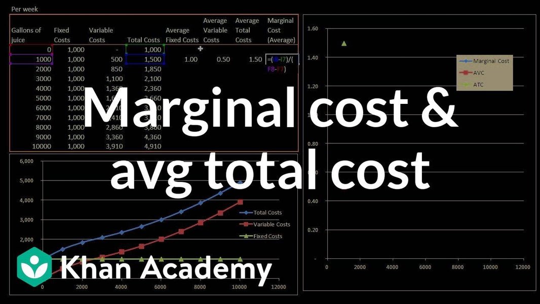
This video by Khan Academy elucidates the calculation of various costs associated with producing a good, including fixed costs, variable costs, marginal cost, and average variable cost. It underscores the dynamic interplay between these cost metrics, emphasizing how marginal cost influences average variable cost. When marginal cost is lower than average variable cost, it pulls the average down; conversely, when it's higher, it pulls the average up. The point where marginal cost equals average variable cost is crucial for optimizing production levels and minimizing costs.

References

Last updated April 10, 2025