Unpacking Bayesian Quantile Regression with Expert Elicitation

Integrating domain expertise into quantile regression via Stan

expert elicitation session with statistical charts

Key Highlights

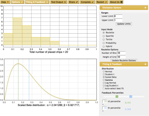
Expert Knowledge Elicitation: Structured protocols capture domain experts' insights into quantile-parameterized prior distributions.
Generalized Asymmetric Laplace Distribution: This flexible distribution is foundational for modeling asymmetry in Bayesian quantile regression.
Stan Implementation: A complete model in Stan facilitates robust estimation using MCMC, where priors and likelihoods are carefully specified.

Overview of the Process

In Bayesian Quantile Regression (BQR), incorporating expert knowledge using a quantile-parameterized prior enhances the regression estimates when empirical data is limited or contains heterogeneity. Here, the generalized asymmetric Laplace distribution (GALD) is utilized as the posterior, which can capture asymmetry and tail behavior robustly. By integrating domain expertise into the prior via elicitation processes, the model becomes more informative and responsive to expert judgments.

Understanding the Components

Expert Knowledge Elicitation

Expert knowledge elicitation involves systematic procedures to extract quantifiable insights from domain experts. These insights—often provided through structured interviews, surveys, or workshops—can be used to define key quantiles (e.g., the median, lower and upper quartiles) of model parameters. The elicited data is transformed into quantile-parameterized distributions (QPDs) that serve as priors, which reflect expert beliefs on model behavior.

Quantile-Parameterized Priors

Quantile-parameterized distributions allow the specification of the distribution based on its quantiles instead of traditional parameters. Experts provide estimates for the desired quantiles, such as the expected median and variability around these points. These quantiles are then mapped onto the parameters of the prior distribution. For Bayesian quantile regression, this approach ensures that the priors align closely with domain-specific expectations.

Generalized Asymmetric Laplace Distribution (GALD)

The generalized asymmetric Laplace distribution is a natural choice for quantile regression because it directly incorporates an asymmetry parameter that dictates the quantile of interest. The GALD is characterized by three main parameters:

Location (mu): Represents the central tendency of the distribution.
Scale (sigma): Controls the spread or dispersion.
Shape (nu): Determines the degree of asymmetry, directly related to the quantile being estimated.

In a likelihood function, the GALD provides an appropriate structure to evaluate how well the observed data aligns with the model assumptions. Its flexibility in modeling asymmetry makes it ideal for situations where the response distribution is not symmetric.

Bayesian Quantile Regression Model with Expert Elicitation in Stan

Step 1: Model Structure and Likelihood

Begin by formulating the Bayesian quantile regression model. This involves defining the response variable as a function of predictors, with the likelihood for each observation modeled using the generalized asymmetric Laplace distribution. Specifically, for a given response variable y and predictor X, the model is represented as:

y ~ GALD(μ, σ, ν)

Where:

μ (location) is modeled as a function of predictor variables.
σ (scale) reflects the dispersion in the response.
ν (shape) is the asymmetry parameter, often representing the quantile of interest (e.g., 0.5 for the median).

Step 2: Eliciting Expert Knowledge

The expert elicitation process is central to setting the priors. The following steps are recommended:

Preparation: Prepare surveys or structured interviews to query experts about the expected quantile behavior of the response variable. Request estimates for key metrics such as the median and variability for specific quantiles.
Quantile Specification: Ask experts for direct estimates of quantiles, for example, “What is the likely median value for the outcome?” and “What are the plausible lower and upper quartiles?”.
Mapping to Parameters: Use the elicited quantiles to derive parameters for the prior distributions associated with μ, σ, and ν. This may involve constructing distributions such as the normal or inverse gamma with parameters set to reflect expert insights.
Quantile-Parameterized Prior Definition: Formulate these priors so that they directly incorporate the quantile estimates. For instance, if experts believe that the median of y is around a specific value with known variability, set:
μ ~ N(y_q0, σ_yq)

Step 3: Implementing the Model in Stan

With the model and priors defined, the next step is to implement the Bayesian quantile regression in Stan. The following is a simplified version of how the code might look:


// Stan model for Bayesian Quantile Regression with Expert Elicitation
data {
  int<lower=0> N;         // Number of observations
  int<lower=0> K;         // Number of predictors
  vector[N] y;            // Response variable
  matrix[N, K] X;         // Predictor matrix
  real q;                 // Desired quantile (e.g., 0.5 for the median)
  // Expert elicited hyperparameters
  real y_q0;              // Expert's median estimate for y at quantile q
  real sigma_yq;          // Spread around the quantile estimate
  real a;                 // Parameters for the InvGamma prior for sigma
  real b;
  real nu0;               // Expert-specified mean for the asymmetry parameter
  real sigma_nu;          // Spread for the asymmetry parameter
}

parameters {
  vector[K] beta;       // Regression coefficients
  real<lower=0> sigma;    // Scale parameter
  real nu;                // Shape/asymmetry parameter, related to q
}

model {
  // Expert informed priors
  // Specify the location parameter using the elicited quantile for y
  // Here, the linear predictor X * beta represents the median (for q=0.5) or other quantile
  beta ~ normal(0, 10);   // Default weakly informative prior; replace with elicited values if available
  sigma ~ inv_gamma(a, b);
  nu ~ normal(nu0, sigma_nu);

  // Likelihood using a generalized asymmetric Laplace distribution 
  // The likelihood function is constructed using the asymmetric Laplace which can be parameterized in Stan
  for (i in 1:N) {
    y[i] ~ custom_asym_laplace_lpdf(X[i] * beta | sigma, nu, q);
  }
}

In this code snippet, the function custom_asym_laplace_lpdf is assumed to implement the log-density of the generalized asymmetric Laplace distribution based on the parameters provided. In practice, a user would define or utilize an existing implementation that computes this density accurately.

Step 4: Model Validation and Sensitivity Analysis

After fitting the model using Markov Chain Monte Carlo (MCMC) methods in Stan, carry out a posterior analysis to understand how well the elicited expert knowledge and other priors are influencing the estimates. This involves:

Comparing the posterior distributions of the regression coefficients, the scale, and the asymmetry parameters against expert expectations.
Calculating predictive checks such as the mean absolute error (MAE) or mean squared error (MSE) using generated quantities in Stan.
Conducting sensitivity analyses by varying hyperparameters to assess the robustness of the model to changes in the elicited priors.

The validation process ensures that the integration of expert knowledge meaningfully enhances the model and does not simply over-constrain it.

Comprehensive Model Summary Table

Component	Description	Example Prior or Parameter
Expert Knowledge Elicitation	Structured protocol to extract domain expert insights on key quantiles.	Quantiles: Median, Lower Quartile, Upper Quartile
Quantile-Parameterized Priors	Priors specified in terms of elicited quantiles to inform model parameters.	\( \mu \sim N(y_{q0}, \sigma_{yq}) \)
Likelihood Function	Modeled using the generalized asymmetric Laplace distribution to capture asymmetry and quantile-specific behavior.	y ~ GALD(μ, σ, ν, q)
Stan Implementation	Custom Stan code incorporating expert priors, likelihood using GALD, and MCMC for inference.	See Stan code snippet above
Model Validation	Posterior and sensitivity analyses to evaluate model fit and robustness.	MAE, MSE estimates from generated quantities

Additional Considerations

Incorporating expert knowledge into Bayesian quantile regression is not only a statistical exercise but also involves carefully managing uncertainties inherent in subjective judgments. While the above approach outlines the structural steps in the context of Stan, practitioners should consider:

Detailed calibration sessions with experts to refine quantile estimates.
Use of probabilistic models to bridge expert elicitation and statistical inference.
Iterative model adjustments and sensitivity tests to mitigate overconfidence in elicited priors.

This methodology ultimately improves the reliability of estimates in contexts where limited data might otherwise undermine model confidence.