
Calculating Partial Overlap Between Two Hermite Functions
A Comprehensive Guide to Understanding and Computing Partial Overlaps
Key Takeaways
- Hermite functions are orthonormal and play a crucial role in quantum mechanics and signal processing.
- Partial overlap quantifies the inner product of two Hermite functions over a finite interval, differing from complete orthonormality.
- Both analytical and numerical methods are essential for calculating partial overlaps, with numerical integration often being the practical choice.
Introduction to Hermite Functions
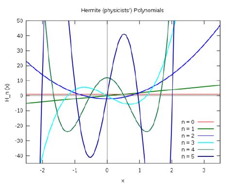
Hermite functions are a set of orthonormal functions derived from Hermite polynomials. They are widely used in various fields including quantum mechanics, particularly in the study of the quantum harmonic oscillator, and signal processing due to their favorable mathematical properties. The orthonormality of Hermite functions makes them an essential tool for expanding functions in series, akin to Fourier series.
Definition and Properties
The normalized one-dimensional Hermite functions, denoted as \(\psi_n(x)\), are defined by the formula:
\[ \psi_n(x) = \frac{1}{\sqrt{2^n n! \sqrt{\pi}}} e^{-x^2/2} H_n(x) \]where \(H_n(x)\) represents the Hermite polynomials of degree \(n\). These functions satisfy the orthonormality condition:
\[ \int_{-\infty}^{\infty} \psi_n(x) \psi_m(x) \, dx = \delta_{nm} \]Here, \(\delta_{nm}\) is the Kronecker delta, which equals 1 when \(n = m\) and 0 otherwise. This property is fundamental in ensuring that Hermite functions form an orthonormal basis in the space \(L^2(\mathbb{R})\).
Understanding Partial Overlap
The concept of partial overlap refers to the evaluation of the inner product between two Hermite functions over a finite interval, as opposed to the entire real line. While complete orthonormality considers the integration over \(-\infty\) to \(\infty\), partial overlap examines how much the two functions overlap within a specific finite range [\(a\), \(b\)].
Mathematical Formulation
The partial overlap between two Hermite functions \(\psi_n(x)\) and \(\psi_m(x)\) is quantified by the integral:
\[ O_{nm}(a, b) = \int_{a}^{b} \psi_n(x) \psi_m(x) \, dx \]This integral measures the inner product of the two functions within the interval [\(a\), \(b\)]. Unlike the complete overlap, which simplifies to the Kronecker delta due to orthonormality, the partial overlap depends on the specific limits \(a\) and \(b\), as well as the indices \(n\) and \(m\) of the Hermite functions involved.
Analytical Approaches to Calculating Partial Overlap
In certain cases, especially when dealing with low-order Hermite functions and specific intervals, it is possible to evaluate the partial overlap integral analytically. This requires leveraging the properties of Hermite polynomials and Gaussian integrals.
Example of Analytical Calculation
Consider calculating the partial overlap between \(\psi_0(x)\) and \(\psi_1(x)\) over the interval [0, 1]. The Hermite functions in this case are:
\[ \psi_0(x) = \frac{1}{\pi^{1/4}} e^{-x^2/2}, \quad \psi_1(x) = \frac{\sqrt{2}}{\pi^{1/4}} x e^{-x^2/2} \]The partial overlap integral becomes:
\[ O_{01}(0, 1) = \int_{0}^{1} \psi_0(x) \psi_1(x) \, dx = \frac{\sqrt{2}}{\pi^{1/2}} \int_{0}^{1} x e^{-x^2} \, dx \]This integral can be evaluated analytically by performing a substitution:
\[ \int x e^{-x^2} \, dx = -\frac{1}{2} e^{-x^2} + C \]Applying the limits from 0 to 1:
\[ O_{01}(0, 1) = \frac{\sqrt{2}}{2\pi^{1/2}} \left(1 - e^{-1}\right) \]This provides a precise value for the partial overlap between the two Hermite functions within the specified interval.
Numerical Methods for Partial Overlap Calculation
For most practical applications, especially when dealing with higher-order Hermite functions or arbitrary integration limits, analytical solutions become intractable. In such scenarios, numerical integration methods are employed to approximate the partial overlap integral.
Common Numerical Integration Techniques
- Gaussian Quadrature: Particularly Gauss-Hermite quadrature, is highly efficient for integrals involving Gaussian weight functions.
- Simpson's Rule: A method that approximates the integral by fitting parabolas to segments of the integrand.
- Trapezoidal Rule: Approximates the integral by dividing the area under the curve into trapezoids.
Implementation Using Python
Symbolic Integration with SymPy
Symbolic computation libraries like SymPy can be used to attempt analytical integration of the partial overlap. Below is an example:
import sympy as sp

# Define symbols
x = sp.Symbol('x')
n, m = 0, 1  # Example indices
a, b = 0, 1  # Integration limits

# Define Hermite functions
def hermite_func(n, x):
    Hn = sp.hermite(n, x)
    return (sp.exp(-x<b>2 / 2) * Hn) / sp.sqrt(2</b>n * sp.factorial(n) * sp.sqrt(sp.pi))

psi_n = hermite_func(n, x)
psi_m = hermite_func(m, x)

# Define the integrand
integrand = psi_n * psi_m

# Perform integration
overlap = sp.integrate(integrand, (x, a, b))
print(overlap)
This script attempts to symbolically compute the integral, which may not always yield a closed-form solution for arbitrary \(n\) and \(m\).
Numerical Integration with SciPy
For cases where symbolic integration is infeasible, numerical methods provide a practical alternative. The following example uses SciPy's quad function:
from scipy.special import eval_hermite
from scipy.integrate import quad
import numpy as np

# Define Hermite function
def hermite_func(n, x):
    return np.exp(-x<b>2 / 2) * eval_hermite(n, x) / np.sqrt(2</b>n * np.math.factorial(n) * np.sqrt(np.pi))

# Parameters
n, m = 2, 3  # Example indices
a, b = -1, 1  # Integration limits

# Define the integrand
def integrand(x):
    return hermite_func(n, x) * hermite_func(m, x)

# Perform numerical integration
result, error = quad(integrand, a, b)
print(f"Partial Overlap O_{{{n}{m}}}({a}, {b}) = {result} with error {error}")
This script numerically evaluates the partial overlap between the specified Hermite functions over the given interval.
Choosing the Right Numerical Method
The choice of numerical integration technique depends on the specific requirements of the problem, such as the desired accuracy and computational efficiency:
| Method | Pros | Cons |
|---|---|---|
| Gaussian Quadrature | High accuracy with fewer function evaluations, especially for weight functions similar to Hermite functions. | Requires precomputed nodes and weights, less flexible for arbitrary integrands. |
| Simpson's Rule | Simple to implement, good for smooth integrands. | Less efficient for highly oscillatory or complex integrands. |
| Trapezoidal Rule | Easy to understand and implement, suitable for functions with linear behavior. | Lower accuracy for functions with curvature, may require more subdivisions. |
Step-by-Step Implementation
1. Define the Hermite Functions
First, specify the orders \(n\) and \(m\) of the Hermite functions involved in the calculation. Using these, define \(\psi_n(x)\) and \(\psi_m(x)\) using the Hermite polynomial expressions.
2. Specify the Integration Limits
Determine the finite interval [\(a\), \(b\)] over which the partial overlap is to be calculated. These limits are crucial as they define the region of integration.
3. Choose an Integration Method
Select an appropriate numerical integration technique based on the problem's requirements. For Hermite functions, Gaussian quadrature is often advantageous due to the Gaussian weight in their definition.
4. Perform the Integration
Execute the chosen numerical method to evaluate the integral \(O_{nm}(a, b)\). This can be achieved using programming languages like Python, leveraging libraries such as SciPy and NumPy for efficiency.
5. Interpret the Results
Analyze the computed partial overlap to understand the extent of the interaction between the two Hermite functions within the specified interval. This information can be pivotal in applications like quantum mechanics where such overlaps relate to transition probabilities.
Practical Considerations
When calculating partial overlaps between Hermite functions, several practical factors must be accounted for to ensure accuracy and efficiency:
-
Numerical Precision: Higher-order Hermite functions exhibit more oscillatory behavior, necessitating higher numerical precision and finer integration subdivisions to capture their features accurately.
-
Computational Resources: Intensive calculations, especially for large \(n\) and \(m\), may require substantial computational resources and optimized algorithms.
-
Function Behavior: Understanding the properties of the Hermite functions involved, such as their asymptotic behavior and orthogonality, can inform the choice of integration method and parameter settings.
Conclusion
Calculating the partial overlap between two Hermite functions is a fundamental task in various scientific and engineering disciplines. While analytical solutions are attainable for specific cases, numerical integration methods offer the flexibility and practicality required for more complex scenarios. By carefully defining the Hermite functions, selecting appropriate integration limits and methods, and considering practical computational aspects, one can accurately quantify the partial overlap, thereby gaining deeper insights into the behavior and interactions of these fundamental functions.
References
Last updated January 18, 2025