Unveiling Calibrated Geometry: Where Differential Forms Meet Volume Minimization

A deep dive into the elegant theory connecting minimal surfaces, special holonomy, and theoretical physics.

Calibrated geometry offers a powerful lens through which to view and understand special types of submanifolds within broader geometric spaces. Introduced by Reese Harvey and H. Blaine Lawson in 1982, this field elegantly uses differential forms to identify and characterize submanifolds that minimize volume in a very strong sense. It bridges classical ideas from minimal surface theory with modern concepts in complex geometry, special holonomy, and even string theory.

Highlights of Calibrated Geometry

Volume Minimization via Forms: At its heart, calibrated geometry uses special differential forms (calibrations) to single out submanifolds that are absolute volume minimizers within their homology class.
Deep Ties to Special Holonomy: The theory is intrinsically linked to manifolds with special holonomy groups (like Calabi-Yau, G₂ , and Spin(7)), where naturally occurring parallel forms serve as calibrations.
Rich Interdisciplinary Connections: Calibrated geometry finds applications and connections in complex and symplectic geometry, gauge theory, geometric analysis, and theoretical physics, particularly string/M-theory.

What is Calibrated Geometry?

Imagine exploring a curved space (a Riemannian manifold) and wanting to find surfaces or higher-dimensional objects within it that are "tight" or "efficient" in terms of their volume or area. Calibrated geometry provides a sophisticated toolkit for identifying such objects.

The Core Idea: Calibrations and Volume Minimization

The central concept is that of a calibration. Consider a Riemannian manifold \((M, g)\) of dimension \(n\), where \(g\) is the metric measuring distances and angles. A calibration is a specific type of differential \(p\)-form \(\varphi\) (where \(0 \le p \le n\)) defined on \(M\). This form must satisfy two crucial properties:

Closedness: The form must be closed, meaning its exterior derivative is zero: \[ d\varphi = 0 \] This condition is essential, linking the theory to cohomology and conservation laws via Stokes' theorem.
Comass Condition: For any point \(x \in M\) and any oriented \(p\)-dimensional tangent subspace \(\xi \subseteq T_x M\), the restriction of the form \(\varphi\) to \(\xi\) must be less than or equal to the volume form induced by the metric \(g\) on \(\xi\). Mathematically, \[ \varphi|_{\xi} \le \text{vol}_{\xi} \] This is often stated by saying the "comass" of \(\varphi\) is less than or equal to 1.

A \(p\)-dimensional submanifold \(N \subseteq M\) is then called calibrated by \(\varphi\) if, at every point \(x \in N\), the restriction of \(\varphi\) to the tangent space \(T_x N\) achieves the maximum possible value; that is, it equals the volume form:

\[ \varphi|_{T_x N} = \text{vol}_{T_x N} \quad \text{for all } x \in N \]

The power of this definition lies in a fundamental theorem: Any calibrated submanifold is automatically volume-minimizing within its homology class. This means that if you take any other submanifold \(N'\) that represents the same "hole" in the manifold \(M\) (i.e., \(N\) and \(N'\) are homologous), then the volume of \(N\) is less than or equal to the volume of \(N'\). This is a much stronger condition than just being a minimal submanifold (which only requires zero mean curvature, a local condition). Calibrated submanifolds are *absolute* minimizers.

Foundational Work by Harvey and Lawson

The framework of calibrated geometry was systematically developed in the seminal 1982 paper "Calibrated Geometries" by Reese Harvey and H. Blaine Lawson Jr. Their work provided a unified perspective on various known examples of volume-minimizing submanifolds (like complex submanifolds in Kähler manifolds) and opened the door to discovering new ones, particularly in the context of manifolds with special geometric structures (special holonomy).

Key Examples and Connections

Calibrated geometry is not an isolated theory; it thrives on its connections to other areas of geometry and physics. Some of the most important examples arise naturally in specific geometric settings.

Complex and Kähler Geometry

One of the earliest and most fundamental examples comes from Kähler geometry. A Kähler manifold is a complex manifold equipped with a compatible Riemannian metric and a symplectic form (the Kähler form \(\omega\)).

Visual representation of a Riemannian submanifold

Conceptual illustration related to submanifolds in geometric spaces.

The Kähler Form as a Calibration

The Kähler form \(\omega\) itself (or powers of it, \(\omega^k / k!\) for \(2k\)-dimensional submanifolds) acts as a calibration. The submanifolds calibrated by \(\omega^k / k!\) are precisely the \(k\)-dimensional complex submanifolds of the ambient Kähler manifold. This recovers the classical result by Wirtinger that complex submanifolds are volume-minimizing.

Manifolds with Special Holonomy

Perhaps the richest source of examples comes from Riemannian manifolds whose holonomy group (the group capturing how tangent vectors change when parallel transported around closed loops) is a special subgroup of the orthogonal group \(SO(n)\). These manifolds possess parallel differential forms, which are automatically closed (\(d\varphi = 0\)) and often serve as calibrations.

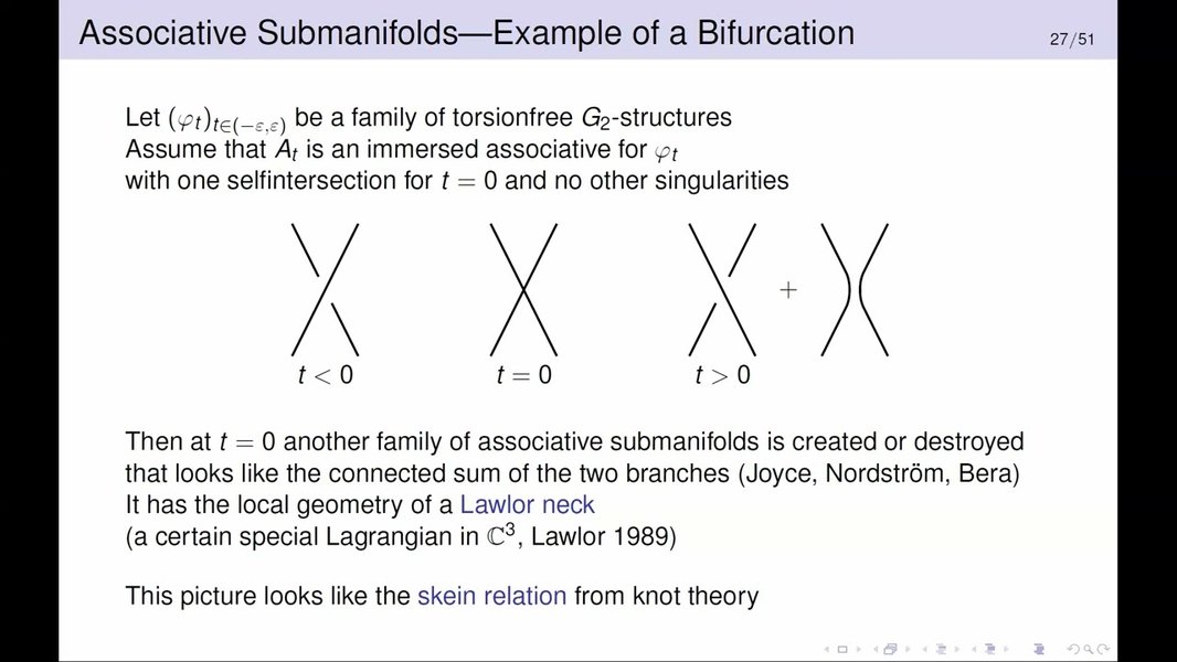
Research talks often delve into specific types of special holonomy, like G₂-manifolds.

Calabi-Yau Manifolds and Special Lagrangians

Calabi-Yau manifolds are Kähler manifolds with Ricci curvature zero and holonomy group contained in \(SU(m)\) (where \(n=2m\) is the real dimension). They admit a parallel holomorphic volume form \(\Omega\). The real part, \(\text{Re}(\Omega)\), acts as a calibration for \(m\)-dimensional submanifolds. The calibrated submanifolds are called Special Lagrangian (SLag) submanifolds. These are Lagrangian submanifolds (meaning the Kähler form \(\omega\) restricts to zero on them) satisfying an additional phase condition related to \(\Omega\). SLag submanifolds are crucial objects in mirror symmetry and string theory.

G₂ Manifolds: Associative and Coassociative Submanifolds

In 7 dimensions, manifolds with the exceptional holonomy group G₂ possess a parallel 3-form \(\varphi\) and its Hodge dual, a parallel 4-form \(*\varphi\).

The 3-form \(\varphi\) calibrates 3-dimensional submanifolds called associative submanifolds.
The 4-form \(*\varphi\) calibrates 4-dimensional submanifolds called coassociative submanifolds.

These play significant roles in M-theory compactifications.

Spin(7) Manifolds and Cayley Submanifolds

In 8 dimensions, manifolds with the exceptional holonomy group Spin(7) admit a parallel, self-dual 4-form \(\Phi\), known as the Cayley form. This form calibrates 4-dimensional submanifolds called Cayley submanifolds. These are also important in theoretical physics contexts.

Symplectic Geometry Links

Calibrated geometry also connects to symplectic geometry, particularly through Lagrangian submanifolds. Special Lagrangian submanifolds in Calabi-Yau manifolds are a prime example. The study of volume-minimizing Lagrangian cycles is an active area where calibrated techniques can be applied.

Deeper Theoretical Aspects

Beyond specific examples, calibrated geometry involves rich theoretical structures and analytical properties.

Stability and Volume Minimization Properties

As mentioned, calibrated submanifolds are absolute volume minimizers in their homology class. This implies they are stable minimal submanifolds. Studying the second variation of volume confirms their stability. The theory provides a powerful criterion (checking if \(\varphi|_{TN} = \text{vol}_{TN}\)) for identifying these highly stable, volume-minimizing objects.

Geometric Flows and Deformations

Calibrated submanifolds often arise as stationary points or stable limits of geometric evolution equations, such as the Mean Curvature Flow. For instance, the Lagrangian Mean Curvature Flow (LMCF) studies how Lagrangian submanifolds evolve under mean curvature. Special Lagrangian submanifolds are fixed points of this flow. Understanding the dynamics of these flows near calibrated submanifolds is a key research direction.

Potential Theory in Calibrated Geometry

Recent research has extended concepts from complex potential theory (like plurisubharmonic functions) to the setting of calibrated geometry. For a calibration \(\varphi\), one can define \(\varphi\)-plurisubharmonic functions as functions whose restriction to any calibrated plane is subharmonic. This allows for the definition of \(\varphi\)-pseudo-convex domains and the application of analytical tools to study the geometry and topology of calibrated manifolds and their submanifolds.

Applications Beyond Pure Mathematics

The impact of calibrated geometry extends significantly into theoretical physics, particularly in the context of string theory, M-theory, and gauge theory.

Gauge Theory and Theoretical Physics

In string theory and M-theory, spacetime is often modeled as a product of our familiar 4-dimensional spacetime and a compact higher-dimensional manifold (e.g., a Calabi-Yau, G₂, or Spin(7) manifold). Physical objects like D-branes or M-branes wrapping cycles in this internal manifold must often minimize energy or volume to preserve supersymmetry.

Supersymmetric Cycles

Calibrated submanifolds often correspond precisely to these supersymmetric cycles. For instance:

D-branes in Type II string theory wrapping special Lagrangian cycles in Calabi-Yau manifolds preserve some supersymmetry.
M-branes wrapping associative or coassociative cycles in G₂ manifolds, or Cayley cycles in Spin(7) manifolds, also preserve supersymmetry in M-theory compactifications.

This connection makes calibrated geometry an indispensable tool for constructing physically realistic string/M-theory models.

Connections to Instantons

Furthermore, calibrated geometry connects to gauge theory constructions like instantons (solutions to Yang-Mills equations) on these special holonomy manifolds. For example, instantons on associative or coassociative submanifolds within G₂ manifolds are studied.

Video Exploration: Gauge Theory and Calibrated Geometry

The interplay between gauge theory and calibrated geometry is a deep and active area of research. This connection highlights how abstract geometric structures find concrete relevance in theoretical physics frameworks. The following video features Gang Tian discussing these connections, offering insights into how these fields inform each other.

Understanding these links requires knowledge of both differential geometry (manifolds, forms, connections) and theoretical physics concepts (supersymmetry, branes, gauge fields). Calibrated submanifolds provide geometrically preferred locations for physical objects and phenomena within higher-dimensional theories.

Comparative Overview of Calibrated Submanifolds

Different types of calibrated submanifolds arise in various geometric contexts, each with unique characteristics. The radar chart below provides a comparative, qualitative assessment of some key examples based on several criteria. Note that these ratings are subjective interpretations for illustrative purposes.

This chart highlights the diversity within calibrated geometry. Complex submanifolds are intimately tied to Kähler geometry, while SLag, Associative, Coassociative, and Cayley submanifolds are characteristic of special holonomy settings in specific dimensions, finding strong applications in modern theoretical physics. Their geometric complexity also tends to increase in these exceptional cases.

Conceptual Map of Calibrated Geometry

The following mind map illustrates the core concepts of calibrated geometry and their interrelationships, showing how the fundamental definitions lead to key examples and applications.

mindmap root["Calibrated Geometry"] id1["Core Concepts"] id1a["Riemannian Manifold (M, g)"] id1b["Calibration Form φ"] id1b1["p-form"] id1b2["Closed (dφ = 0)"] id1b3["Comass ≤ 1
(φ|ξ ≤ volξ)"] id1c["Calibrated Submanifold N"] id1c1["Tangent spaces T<0xE1><0xB5><0xBD>N are calibrated
(φ|T<0xE1><0xB5><0xBD>N = vol<0xE2><0x82><0x99><0xE1><0xB5><0xBD>N)"] id1c2["Volume Minimizing
in Homology Class"] id1c3["Minimal Submanifold
(Mean Curvature = 0)"] id2["Key Examples & Settings"] id2a["Kähler Manifolds"] id2a1["Calibration: Kähler form ω
(or ω<0xE1><0xB5><0x83>/k!)"] id2a2["Calibrated: Complex Submanifolds"] id2b["Special Holonomy Manifolds"] id2b1["Calabi-Yau (SU(m))"] id2b1a["Calibration: Re(Ω)"] id2b1b["Calibrated: Special Lagrangian (SLag)"] id2b2["G₂ Manifolds"] id2b2a["Calibration: φ (3-form)"] id2b2b["Calibrated: Associative (3D)"] id2b2c["Calibration: *φ (4-form)"] id2b2d["Calibrated: Coassociative (4D)"] id2b3["Spin(7) Manifolds"] id2b3a["Calibration: Φ (4-form)"] id2b3b["Calibrated: Cayley (4D)"] id3["Connections & Applications"] id3a["Differential Geometry"] id3a1["Minimal Surface Theory"] id3a2["Geometric Analysis"] id3a3["Geometric Flows (MCF, LMCF)"] id3b["Theoretical Physics"] id3b1["String Theory / M-Theory"] id3b2["Supersymmetric Cycles (Branes)"] id3b3["Gauge Theory (Instantons)"] id3c["Symplectic Geometry"] id3c1["Lagrangian Submanifolds"] id3d["Potential Theory"] id3d1["φ-plurisubharmonic functions"]

This map shows the central role of the calibration form \(\varphi\) and its properties, leading to the definition of calibrated submanifolds which minimize volume. These concepts find concrete realizations in Kähler geometry and, most notably, in manifolds with special holonomy, which in turn connect deeply to theoretical physics and other areas of geometry.

Summary Table of Key Calibrated Submanifolds

The following table summarizes the primary examples of calibrated submanifolds discussed, particularly those arising from special holonomy.

Type of Submanifold	Dimension (p)	Ambient Manifold Type	Ambient Dimension (n)	Calibration Form	Holonomy Group
Complex Submanifold	\(2k\)	Kähler	\(2m\) (\(k \le m\))	\(\omega^k / k!\)	\(U(m)\)
Special Lagrangian (SLag)	\(m\)	Calabi-Yau	\(2m\)	\(\text{Re}(\Omega)\)	\(SU(m)\)
Associative	3	G₂ Manifold	7	\(\varphi\) (3-form)	G₂
Coassociative	4	G₂ Manifold	7	\(*\varphi\) (4-form)	G₂
Cayley	4	Spin(7) Manifold	8	\(\Phi\) (4-form)	Spin(7)

This table underscores the tight relationship between the type of calibrated submanifold, the dimension, the geometry of the ambient space (often characterized by its holonomy group), and the specific differential form acting as the calibration.

Frequently Asked Questions (FAQ)

What exactly is a calibration form?

A calibration form \(\varphi\) is a differential \(p\)-form on a Riemannian manifold \((M, g)\) that satisfies two conditions: it must be closed (\(d\varphi = 0\)), and its value on any oriented \(p\)-dimensional tangent plane \(\xi\) must be less than or equal to the volume of that plane (\(\varphi|_{\xi} \le \text{vol}_{\xi}\)). Think of it as a differential form designed to "measure" \(p\)-dimensional planes, giving a maximum value of 1 (relative to the volume) only for specific "calibrated" orientations.

Are all minimal submanifolds calibrated?

No. While every calibrated submanifold is a minimal submanifold (meaning it has zero mean curvature), the converse is not true. Being calibrated is a stronger condition. It implies not just local volume stationarity (minimality) but absolute volume minimization within the homology class. There exist minimal submanifolds that cannot be calibrated by any calibration form on the ambient manifold.

Why is calibrated geometry important in physics?

Calibrated geometry is crucial in string theory and M-theory, particularly in models involving extra spatial dimensions (compactification). Physical objects like D-branes or M-branes often wrap cycles (submanifolds) in these extra dimensions. To preserve supersymmetry (a key theoretical principle), these branes must often wrap calibrated cycles. This is because calibrated submanifolds minimize volume (or energy), which is typically required for stability and supersymmetry. Examples include Special Lagrangians in Calabi-Yau manifolds, Associative/Coassociative cycles in G₂ manifolds, and Cayley cycles in Spin(7) manifolds.

What background is needed to study calibrated geometry?

A solid foundation in differential geometry is essential. This includes understanding manifolds, tangent spaces, Riemannian metrics, differential forms, exterior derivatives, Stokes' theorem, and connections/curvature. Familiarity with basic concepts from algebraic topology (like homology) is also very helpful, as volume minimization is often stated relative to homology classes. For specific areas, knowledge of complex geometry (Kähler manifolds) or representation theory (for special holonomy groups like G₂ and Spin(7)) is necessary.

References

image-engineering.de
Last updated April 29, 2025