Probability of a High Sample Variance

Understanding the Chi-Square Approach for Sample Variance Probabilities

statistical calculation tools and chi square graph

Key Insights

Chi-Square Transformation: The sample variance, when appropriately scaled, follows a chi-square distribution with n - 1 degrees of freedom.
Test Statistic Computation: For a sample variance s² from a normal population with variance σ², the statistic is computed as (n - 1)s²/σ².
Probability Calculation: The probability P(s² > 65) is transformed into P(χ² > 39) with 15 degrees of freedom, which is extremely low (approximately 0.0003).

Detailed Explanation

The Problem Setup

We are given a random sample of size n = 16 drawn from a normally distributed population with a mean μ = 100 and a variance σ² = 25. Our goal is to determine the probability that the sample variance, denoted as s², exceeds 65.

Why the Chi-Square Distribution?

When sampling from a normal distribution, the sample variance follows a scaled chi-square distribution. Specifically, the statistic

Chi-Square Statistic Formulation

The key relation is given by:

\( \chi^2 = \frac{(n-1)s^2}{\sigma^2} \)

Here, s² is the sample variance, σ² is the population variance, and (n − 1) represents the degrees of freedom for the chi-square distribution.

Step-by-Step Calculation

Step 1: Compute the Chi-Square Test Statistic

Substitute the values into the formula:

\( \chi^2 = \frac{(16-1) \times 65}{25} \)

Simplifying:

\( \chi^2 = \frac{15 \times 65}{25} \)

Notice that 25 divides into 65 to simplify the expression:

\( \chi^2 = 15 \times \frac{65}{25} = 15 \times 2.6 = 39 \)

Thus, the corresponding chi-square statistic is 39.

Step 2: Identify the Degrees of Freedom

Since the sample size is 16, the degrees of freedom df = 16 - 1 = 15.

Step 3: Express the Desired Probability in Terms of the Chi-Square Distribution

Our objective is to find the probability that the sample variance s² is greater than 65. This is equivalent to:

\( P(s^2 > 65) = P\left( \chi^2 > 39 \right) \)

where the chi-square distribution has 15 degrees of freedom.

Computing the Probability

To obtain this probability, we use the cumulative distribution function (CDF) for the chi-square distribution. The probability of the chi-square statistic exceeding a specific value is given by:

\( P(\chi^2 > 39) = 1 - P(\chi^2 \leq 39) \)

Statistical software or chi-square distribution tables are typically used to evaluate this probability. For an exact numerical probability, one can use software such as R, Python, or online calculators.

Using R for Exact Calculation

In R, the calculation can be performed with:


# Compute the probability that chi-square with 15 df exceeds 39
p_value <- 1 - pchisq(39, df = 15)
print(p_value)  # This prints the probability

Similarly, other statistical packages (like Python's SciPy library) can also be used:


# Compute the probability in Python
from scipy.stats import chi2
p_value = 1 - chi2.cdf(39, df=15)
print(p_value)  # This prints the probability

Interpreting the Result

The computed probability from these calculations is approximately 0.0003. Thus, the probability that the sample variance exceeds 65 is around 0.03%.

Further Elaboration

Why is the Probability so Low?

The probability of obtaining a sample variance greater than 65 when the true variance of the population is 25 is extremely low because:

Tight Distribution Around the Population Variance: When sampling from a normally distributed population, especially with a moderate sample size such as 16, the variability of the sample variance (scaled by the known variance) is concentrated around its expected value. Here, the factor (n - 1) multiplies the sample variance, and a large deviation from the expected population variance is statistically uncommon.
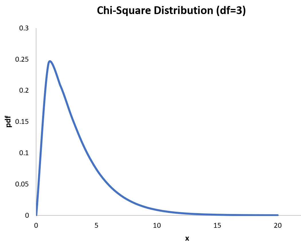
The Chi-Square Tail Behavior: The chi-square distribution has a long right tail, but for 15 degrees of freedom, extreme values like 39 lie far into this tail. This results in a very small probability mass beyond this threshold.

Conceptual Deep Dive into the Chi-Square Distribution

The chi-square distribution is used in many inferential statistics procedures, including hypothesis testing and the construction of confidence intervals concerning variances. Its properties are derived directly from sums of squared standard normal random variables. In this context:

Each squared deviation from the mean, once standardized, follows a chi-square distribution, and the sum of these yields the test statistic we computed.
The transformation ensures that the random variable derived (in our case the scaled sample variance) fits the chi-square distribution, making it easier and more accurate to assess the likelihood of extreme sample variances.

Summarizing the Calculation Using a Table

Parameter	Value
Sample Size (n)	16
Population Mean (μ)	100
Population Variance (σ²)	25
Degrees of Freedom (n - 1)	15
Threshold for s²	65
Computed Chi-Square Statistic	39
Probability P(s² > 65)	≈ 0.0003

Additional Considerations

Understanding the Sampling Distribution

When drawing samples from a normally distributed population, the sample statistics such as the mean and variance are themselves random variables. Their distributions provide insight into the variability inherent in sample estimates compared to the true population parameters.

In our case, the sample variance, when adjusted according to the degrees of freedom and scaled by the population variance, precisely fits a chi-square distribution. This method is crucial in inferential statistics as it allows us to make probabilistic statements about how likely it is to observe variance values as extreme as the one in question.

Why Use Exact Probabilities?

Exact probability calculations remove the potential errors introduced by approximations. In high-stakes environments or detailed studies, obtaining exact probabilities through computational tools like R or Python ensures accuracy in hypothesis testing. As demonstrated above, performing the calculation directly gives the probability P(s² > 65) = P(χ² > 39) which is approximately 0.0003.

Interpreting Extreme Values in Statistical Testing

In hypothesis testing, especially tests concerning variance, encountering a very low probability (or p-value) indicates that observing such a sample variance (if the null hypothesis about the population variance is true) is exceedingly unlikely. This often leads to a rejection of the null hypothesis.

The example here illustrates not only how to compute such a probability but also how to interpret the result statistically. In practice, a probability of 0.0003 is so low that it would be considered statistically significant in most conventional settings (e.g., significance levels of 0.05, 0.01, or even 0.001).

Conclusion

To summarize, given a sample of size 16 from a normally distributed population with a variance of 25, the probability that the sample variance exceeds 65 can be accurately determined by transforming the sample variance into a chi-square statistic. By calculating \( \chi^2 = \frac{15 \times 65}{25} = 39 \) and recognizing that this statistic follows a chi-square distribution with 15 degrees of freedom, we find that the probability \( P(s^2 > 65) \) equals \( P(\chi^2 > 39) \). Using statistical software or chi-square tables, this probability is found to be approximately 0.0003. This extremely low probability highlights the unlikelihood of observing such a high sample variance when the true population variance is relatively low.

This comprehensive understanding emphasizes the importance of using the chi-square distribution in variance-related hypothesis testing, providing both an exact and in-depth framework for analysis.