Understanding and Implementing Merge Sort

Key Insights into Merge Sort

Divide and Conquer: Merge Sort's core principle is to recursively break down an array into smaller subarrays until each contains only one element.
Merging Sorted Subarrays: The crucial step involves merging these single-element subarrays back together in a sorted manner, building larger sorted arrays until the entire original array is sorted.
Consistent Efficiency: Merge Sort boasts a time complexity of O(n log n) in all cases (best, average, and worst), making it a highly reliable sorting algorithm.

What is Merge Sort?

Merge Sort is an efficient, general-purpose, and comparison-based sorting algorithm that follows the divide-and-conquer paradigm. This means it breaks down a large problem into smaller, more manageable subproblems, solves them independently, and then combines their solutions to solve the original problem. In the context of sorting, Merge Sort repeatedly divides an unsorted list or array into two halves until each sublist contains only one element. A single element is inherently sorted.

The "conquer" part of the algorithm involves merging these single-element sublists back together in a sorted order. This merging process is key to the algorithm's efficiency. By repeatedly merging sorted sublists, the algorithm builds larger and larger sorted lists until the entire original list is sorted.

The Divide and Conquer Approach in Detail

The divide and conquer strategy in Merge Sort can be broken down into two primary phases:

The Dividing Phase

In this phase, the algorithm recursively divides the input array into two halves. This process continues until the subarrays can no longer be divided, meaning each subarray contains only one element.

Steps in Dividing:

Start with the unsorted array.
Find the middle point of the array.
Divide the array into two subarrays: from the beginning to the middle, and from the middle + 1 to the end.
Recursively apply the dividing process to both subarrays until each subarray contains only one element.

The Merging Phase

Once the array has been divided into single-element subarrays, the merging phase begins. This phase involves combining the subarrays in a sorted manner.

Steps in Merging:

Take two adjacent sorted subarrays.
Compare the first elements of both subarrays.
Copy the smaller element into a temporary or result array and move the pointer of the subarray from which the element was taken.
Repeat the comparison and copying process until one of the subarrays is empty.
Copy any remaining elements from the non-empty subarray into the result array.
The result array is a new, larger sorted subarray.
This merging process is repeated upwards through the levels of recursion until the original array is fully merged and sorted.

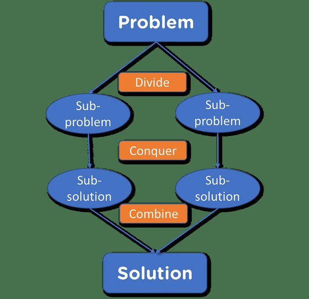
This illustration visually represents the divide and conquer nature of Merge Sort:

Illustration of the Divide and Conquer Principle in Merge Sort

Merge Sort Divide and Conquer Illustration

Implementing Merge Sort (Python Example)

Merge Sort can be implemented in various programming languages. Here's an example implementation in Python, demonstrating both the recursive splitting and the merging process. The implementation typically involves two main functions: one for the recursive splitting (merge_sort) and a helper function for merging the sorted subarrays (merge).

Python Code Implementation:


def merge_sort(arr):
    if len(arr) > 1:
        # Find the middle of the array
        mid = len(arr) // 2
        # Divide the array into two halves
        left_half = arr[:mid]
        right_half = arr[mid:]

        # Recursively sort the two halves
        merge_sort(left_half)
        merge_sort(right_half)

        # Merge the sorted halves
        i = j = k = 0

        # Copy data to temp arrays left_half[] and right_half[]
        while i < len(left_half) and j < len(right_half):
            if left_half[i] < right_half[j]:
                arr[k] = left_half[i]
                i += 1
            else:
                arr[k] = right_half[j]
                j += 1
            k += 1

        # Check for any remaining elements
        while i < len(left_half):
            arr[k] = left_half[i]
            i += 1
            k += 1

        while j < len(right_half):
            arr[k] = right_half[j]
            j += 1
            k += 1

# Example usage:
# if __name__ == '__main__':
#     my_list = [12, 11, 13, 5, 6, 7]
#     merge_sort(my_list)
#     print("Sorted array is:")
#     print(my_list)

This code illustrates the recursive nature of the merge_sort function, which repeatedly divides the input list until it reaches the base case (a list with one element). The merge logic is embedded within the merge_sort function in this specific implementation, handling the comparison and combination of elements from the sorted halves.

Analysis of Merge Sort's Efficiency

One of the most significant advantages of Merge Sort is its predictable performance. Its time complexity is consistently O(n log n) regardless of the initial order of the elements in the input array.

Time Complexity:

The time complexity of Merge Sort can be analyzed by considering the two main steps: division and merging.

Division: The process of repeatedly dividing the array in half takes logarithmic time, specifically O(log n), where 'n' is the number of elements. This is because the depth of the recursion tree is logarithmic with respect to 'n'.
Merging: The merging process at each level of recursion involves comparing and combining 'n' elements (across all the subarrays at that level). This takes linear time, O(n).

Since the merging step of O(n) is performed at each of the O(log n) levels of recursion, the total time complexity is the product of these two: \(O(n \log n)\). This holds true for the best, average, and worst-case scenarios.

Space Complexity:

Merge Sort typically requires O(n) auxiliary space. This is because the merging process requires a temporary array to store the merged elements. While in-place merge sort algorithms exist, they are generally more complex to implement and may have higher constant factors in their time complexity. The O(n) space requirement is a drawback compared to in-place sorting algorithms like QuickSort, which has an average space complexity of O(log n) due to recursion stack space (though its worst-case space complexity can be O(n)).

Stability:

Merge Sort is a stable sorting algorithm. This means that if two elements have the same value, their relative order in the sorted output will be the same as their relative order in the input. This property is important in certain applications, such as sorting data with multiple keys.

Comparison with Other Sorting Algorithms

Understanding Merge Sort's strengths and weaknesses is often best done by comparing it to other common sorting algorithms like QuickSort and HeapSort.

Comparison of Sorting Algorithms
Algorithm	Time Complexity (Worst Case)	Time Complexity (Average Case)	Space Complexity	Stable?
Merge Sort	O(n log n)	O(n log n)	O(n)	Yes
QuickSort	O(n²)	O(n log n)	O(log n) (average), O(n) (worst)	No
HeapSort	O(n log n)	O(n log n)	O(1)	No

As the table shows, Merge Sort's consistent O(n log n) time complexity is a major advantage, particularly in worst-case scenarios where QuickSort can degrade to O(n²). However, Merge Sort's O(n) space complexity is a consideration, especially for memory-constrained environments. HeapSort offers an in-place solution with the same time complexity, but it is not stable.

Applications of Merge Sort

Due to its stability and guaranteed efficiency, Merge Sort is used in various applications, including:

External Sorting: Merge Sort is well-suited for sorting large datasets that do not fit into main memory. The data can be divided into smaller chunks, sorted in memory, and then merged.
Implementations of Standard Sorting Libraries: Variations of Merge Sort, such as TimSort (which is a hybrid sorting algorithm derived from Merge Sort and Insertion Sort), are used in the standard libraries of programming languages like Python, Java, and Swift.
Parallel Processing: The divide-and-conquer nature of Merge Sort makes it easily parallelizable, allowing for faster sorting on multi-core processors.
Counting Inversions: Merge Sort can be adapted to efficiently count the number of inversions in an array. An inversion is a pair of elements that are out of order.

Visualizing Merge Sort

Understanding recursive algorithms like Merge Sort can be challenging without visualization. The process of splitting and merging can be clearly seen through visual aids.

Visual representation of the Merge Sort process

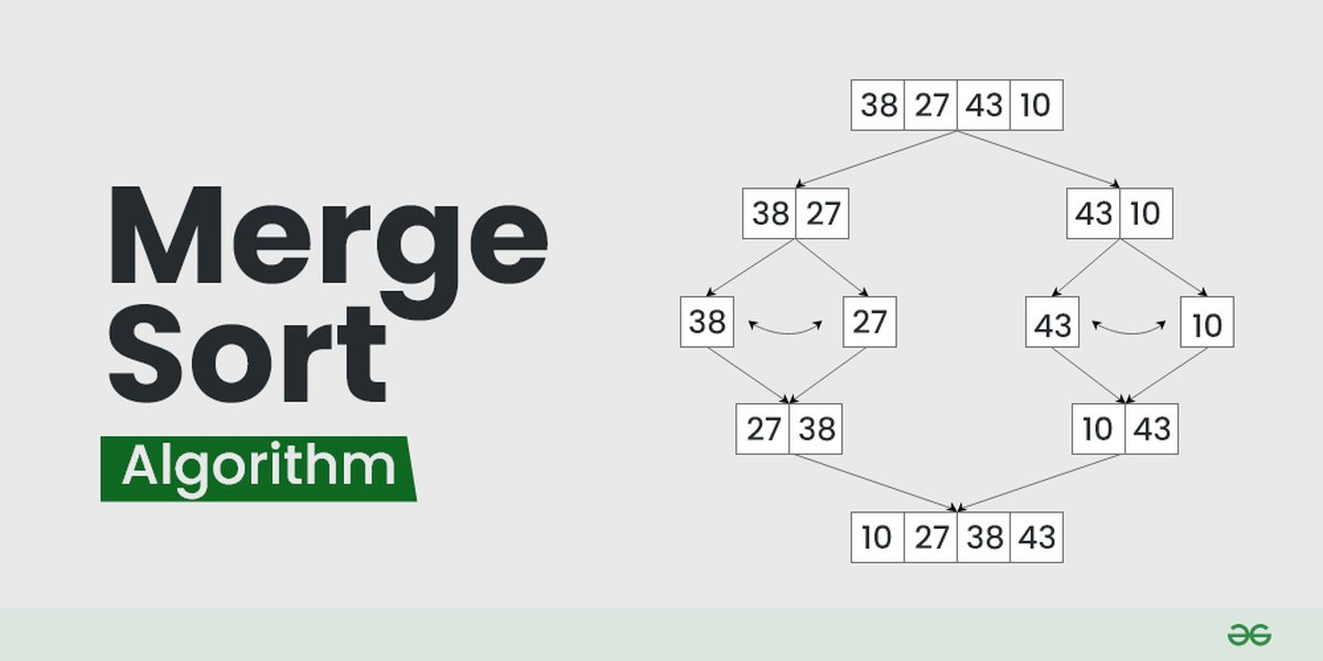
The image above illustrates how the array is recursively divided into smaller subarrays and then merged back together in a sorted order. This step-by-step breakdown helps in grasping the flow of the algorithm.

To further understand the process visually and step-by-step, you can watch the following video which walks through the Merge Sort algorithm:

This video provides a step-by-step walkthrough, helping to solidify your understanding of how the recursion and merging phases interact to sort the data.

Frequently Asked Questions about Merge Sort

Is Merge Sort an in-place sorting algorithm?

Typically, standard implementations of Merge Sort are not in-place as they require O(n) auxiliary space for the merging process. There are variations that attempt to reduce the space complexity, but they are generally more complex.

What is the base case for the recursion in Merge Sort?

The base case for the recursion in Merge Sort is when a subarray contains only one element. A single-element array is considered sorted.

Why is Merge Sort considered a stable sorting algorithm?

Merge Sort is stable because the merging process can be implemented in a way that preserves the relative order of equal elements. When comparing two equal elements from the left and right subarrays during the merge, the element from the left subarray is typically placed first in the merged array, maintaining the original order.

When is Merge Sort preferred over QuickSort?

Merge Sort is preferred over QuickSort when stable sorting is required or when a guaranteed O(n log n) time complexity is necessary, especially in worst-case scenarios. It is also suitable for external sorting.

Can Merge Sort be implemented iteratively?

Yes, Merge Sort can be implemented iteratively (bottom-up) as well as recursively (top-down). The iterative approach starts by merging adjacent single-element subarrays, then adjacent two-element sorted subarrays, and so on, until the entire array is sorted.

References

Last updated May 13, 2025