Unlock Data Integrity: Comparing Spreadsheets and Merging Missing Information

Yes, it is entirely possible to compare data in two spreadsheets, identify information that is missing in one, and then add that missing data from the other. This is a common and crucial task for data management, analysis, and maintaining data integrity, especially when working with large or evolving datasets. Various methods, ranging from simple formulas to powerful built-in tools and specialized software, can accomplish this in spreadsheet applications like Microsoft Excel and Google Sheets.

Key Insights: Streamlining Your Data Comparison

Multiple Methodologies: You can leverage Excel formulas (like COUNTIF, VLOOKUP, XLOOKUP), built-in tools (such as "Consolidate" or "Spreadsheet Compare"), and advanced features like Power Query to find and fill gaps.
Systematic Approach: The process generally involves preparing your data, using a chosen method to identify missing entries by comparing against a reference sheet, and then strategically adding the missing information to the target sheet.
Best Practices Are Crucial: Ensuring data consistency (e.g., uniform unique identifiers), backing up your original files, and understanding your data's structure are vital for accurate and error-free results.

Preparing Your Spreadsheets: The Foundation for Success

Before diving into comparison and merging, proper preparation of your spreadsheets is essential. This groundwork will make the subsequent steps smoother and more accurate.

Ensure Data Consistency

Unique Identifiers

The most critical aspect is having a reliable way to match records between the two sheets. This is typically a column containing unique identifiers (IDs) for each row, such as:

Product SKUs
Employee IDs
Customer Numbers
Email Addresses
Serial Numbers

Ensure these identifiers are consistently formatted in both spreadsheets. For instance, "ID-123" is different from "id123" or "ID 123". Use functions like TRIM to remove extra spaces and ensure consistent casing.

Column Structure

While not strictly necessary for all methods, having a similar or understandable column structure makes the process easier, especially when transferring data. Know which columns correspond to each other in both sheets.

Backup Your Data

Always create backup copies of your original spreadsheets before performing any comparison or merging operations. This protects you from accidental data loss or irreversible changes. Working on copies allows you to experiment with different methods without risking your primary data.

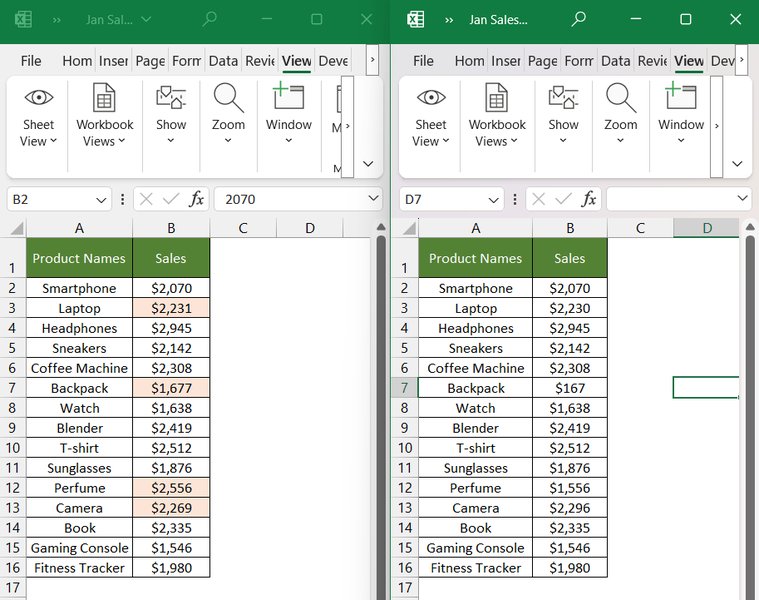
Visual representation of comparing two sheets in Excel

Comparing data side-by-side can be an initial step in identifying differences.

Identifying Missing Information: Uncovering the Gaps

Once your data is prepared, you can use several techniques to pinpoint what's missing in one spreadsheet compared to another. The choice of method often depends on the size of your dataset, your Excel proficiency, and the specific version of Excel or other spreadsheet software you are using.

Using Excel Formulas

Formulas are a flexible way to identify missing records directly within your worksheet.

`COUNTIF` and `IF` Functions

This combination checks if a value from one list exists in another. For example, if you want to check if an ID from Sheet1 (in cell A2) exists anywhere in Column A of Sheet2, you could use this formula in a new column in Sheet1:

=IF(COUNTIF(Sheet2!A:A, A2)=0, "Missing in Sheet2", "Present in Sheet2")

If COUNTIF returns 0, it means the ID from Sheet1!A2 was not found in Sheet2's Column A, indicating it's missing there (or, if comparing the other way, it's an extra item in Sheet1).

`MATCH` and `ISNA` (or `ISNUMBER`) Functions

The MATCH function attempts to find the position of a lookup value within a range. If the value isn't found, it returns an #N/A error. You can use ISNA to test for this error:

=IF(ISNA(MATCH(A2, Sheet2!A:A, 0)), "Missing in Sheet2", "Present in Sheet2")

Here, 0 as the third argument in MATCH specifies an exact match.

`XLOOKUP` or `FILTER` (Modern Excel Versions)

Newer Excel versions (Excel 2021, Microsoft 365) offer more powerful functions. XLOOKUP is a versatile replacement for VLOOKUP/HLOOKUP and can easily check for existence:

=IF(ISERROR(XLOOKUP(A2, Sheet2!A:A, Sheet2!A:A)), "Missing in Sheet2", "Present in Sheet2")

The FILTER function can also be used to return a list of items present in one sheet but not another.

Conditional Formatting

For a visual approach, conditional formatting can highlight cells that are unique to one list or different between two columns. This is useful for quick visual scans but less so for programmatic addition of data.

Microsoft Spreadsheet Compare

If you have Office Professional Plus (2013, 2016, 2019) or Microsoft 365 Apps for enterprise, the "Spreadsheet Compare" tool can analyze two workbooks and highlight differences in values, formulas, and formatting. It provides a report of discrepancies but doesn't automatically merge data.

Adding Missing Information: Bridging the Data Divide

After identifying the missing records, the next step is to populate this information from the source spreadsheet into the target spreadsheet.

Using Lookup Formulas (`VLOOKUP`, `XLOOKUP`)

These are perhaps the most common methods for pulling related data from one sheet to another based on a common identifier.

`VLOOKUP`

If Sheet1 has IDs in Column A and you want to pull corresponding "Product Names" from Sheet2 (where IDs are in Column A and Product Names in Column B) for rows identified as missing this data in Sheet1, you could use:

=IFERROR(VLOOKUP(A2, Sheet2!$A:$B, 2, FALSE), "Data not found in Sheet2")

This formula looks for the ID in Sheet1!A2 within the first column of the range Sheet2!$A:$B, and if found, returns the value from the 2nd column of that range. FALSE ensures an exact match. IFERROR handles cases where the ID might still not be found in Sheet2.

`XLOOKUP`

XLOOKUP simplifies this and is more flexible:

=XLOOKUP(A2, Sheet2!A:A, Sheet2!B:B, "Data not found in Sheet2", 0)

Here, it looks for Sheet1!A2 in Sheet2!A:A, returns the corresponding value from Sheet2!B:B, provides a custom message if not found, and 0 specifies an exact match.

Excel's "Consolidate" Command

The "Consolidate" feature (found on the Data tab) can summarize data from multiple source areas into one destination. While often used for numerical summarization (sum, average), it can also be used to combine lists. You can consolidate by position (if data layouts are identical) or by category (using row and column labels). This is useful for rolling up data from various sheets into a master sheet, potentially bringing in missing rows.

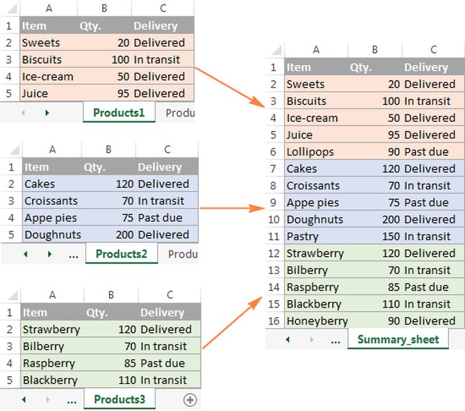
Excel's Consolidate feature can merge data from multiple sheets.

Power Query (Get & Transform Data)

For more complex scenarios, large datasets, or frequent updates, Power Query is an exceptionally powerful tool available in modern Excel versions (and as an add-in for older ones).

Steps with Power Query:

Load Data: Import both spreadsheets (or tables within them) into the Power Query editor.
Merge Queries: Use the "Merge Queries" feature. Select the table that needs data (target) and the table that has the data (source). Choose the common identifier column(s) for both.
Choose Join Kind:
- A "Left Outer Join" (from target to source) will keep all rows from the target and bring in matching data from the source. Rows in the target without a match in the source will have nulls for the source's columns.
- A "Full Outer Join" can show all rows from both tables, helping identify records unique to each.
Expand Data: After merging, expand the column from the source table that contains the data you want to add.
Fill Missing Values: You can then use Power Query's "Fill" commands or conditional columns to populate missing data based on the merged information.
Load to Worksheet: Load the resulting combined and enriched table back into an Excel worksheet.

Power Query steps are refreshable, meaning if your source data changes, you can update the combined table with a click.

Manual Copy and Paste

For very small datasets or one-off tasks where missing items are few and easily identified, manually copying the missing rows or cells from the source sheet and pasting them into the target sheet is feasible. However, this method is prone to errors and not scalable.

Scripting (VBA or Python)

For highly repetitive or complex comparison and merging tasks, scripting languages like VBA (Visual Basic for Applications) within Excel or Python (using libraries like pandas) can automate the entire process. This requires programming knowledge but offers maximum flexibility and efficiency for tailored solutions.

Visualizing Method Effectiveness

Different methods for comparing and adding data excel in different areas. The radar chart below provides a comparative overview of common approaches based on factors like scalability, ease of use for beginners, automation potential, speed for small tasks, and overall versatility.

This chart helps visualize that while manual methods are easy for small, simple tasks, Power Query offers superior scalability and automation for complex, larger datasets. Excel formulas provide a good balance for moderately sized tasks requiring some logic.

Workflow for Data Comparison and Merging

The mindmap below illustrates the typical workflow involved in comparing two spreadsheets, identifying missing information, and adding it from another source. This structured approach helps ensure all necessary steps are considered for effective data reconciliation.

mindmap root["Spreadsheet Data Reconciliation"] id1["1. Preparation Phase"] id1a["Backup Original Files"] id1b["Understand Data Structure"] id1c["Ensure Unique Identifiers (Keys)"] id1d["Clean Data (Trim spaces, Consistent Formatting)"] id2["2. Identify Missing Information"] id2a["Method Selection"] id2a1["Excel Formulas
(COUNTIF, MATCH, XLOOKUP)"] id2a2["Conditional Formatting
(Visual Highlighting)"] id2a3["Spreadsheet Compare Tool"] id2a4["Power Query (Merge & Filter)"] id2a5["Manual Side-by-Side Comparison"] id2b["Execute Comparison"] id2c["Flag or List Missing Records"] id3["3. Add Missing Information"] id3a["Method Selection"] id3a1["Lookup Formulas
(VLOOKUP, XLOOKUP)"] id3a2["Power Query (Merge & Expand)"] id3a3["Excel Consolidate Feature"] id3a4["Manual Copy & Paste (Small Scale)"] id3a5["Scripting (VBA, Python)"] id3b["Transfer Data from Source to Target"] id3c["Handle 'Not Found' Cases"] id4["4. Verification & Finalization"] id4a["Review Merged Data for Accuracy"] id4b["Convert Formulas to Values (Optional)"] id4c["Save Finalized Spreadsheet"]

This mindmap visually breaks down the process into key phases: preparation, identification of missing data, methods for adding that data, and finally, verification to ensure accuracy and completeness.

Key Excel Functions and Tools Summary

The following table summarizes some of the most commonly used Excel functions and tools for comparing spreadsheets and merging data, along with their primary purpose in this context.

Function/Tool	Primary Purpose for Comparison/Merging	Example Use Case
`COUNTIF(range, criteria)`	Checks if an item from one list exists in another list.	`=IF(COUNTIF(Sheet2!A:A, Sheet1!A2)=0, "Missing", "Exists")` to flag items in Sheet1!A2 not found in Sheet2 Column A.
`MATCH(lookup_value, lookup_array, [match_type])`	Finds the relative position of an item in a range; returns #N/A if not found.	Used with `ISNA`: `=IF(ISNA(MATCH(Sheet1!A2, Sheet2!A:A, 0)), "Missing", "Exists")`.
`VLOOKUP(lookup_value, table_array, col_index_num, [range_lookup])`	Looks for a value in the first column of a table and returns a value in the same row from a specified column.	`=VLOOKUP(Sheet1!A2, Sheet2!A:C, 3, FALSE)` to find ID from Sheet1!A2 in Sheet2 Col A and return corresponding data from Sheet2 Col C.
`XLOOKUP(lookup_value, lookup_array, return_array, [if_not_found], [match_mode], [search_mode])`	Modern replacement for VLOOKUP; more flexible and powerful for finding and returning data.	`=XLOOKUP(Sheet1!A2, Sheet2!A:A, Sheet2!C:C, "Not Found")` to get data from Sheet2 Col C based on Sheet1!A2.
Power Query (Get & Transform Data)	Robust tool for importing, transforming, merging, and appending data from various sources, including other sheets or files.	Merging two tables based on a common ID column, performing left/right/full outer joins to identify and combine matching/missing rows.
Consolidate Tool (Data Tab)	Summarizes data from multiple ranges or sheets into a single output range, can be used to combine lists.	Combining sales data from regional sheets into a master sheet, including any unique regions from one sheet not present in others.
Spreadsheet Compare Tool	Compares two workbooks and highlights differences in values, formulas, and formatting.	Identifying all changes between two versions of a financial report. (Requires specific Office versions).

Automating with Power Query: A Deeper Dive

For users who frequently need to combine or update spreadsheets, Power Query offers a robust and automatable solution. The video below provides an excellent tutorial on how to leverage Power Query (often referred to as "Get & Transform Data" in Excel) to combine data from multiple Excel files, a process very similar to combining sheets and identifying/adding missing data.

This video demonstrates how to use Power Query to combine multiple Excel files, showcasing techniques applicable to merging data and handling discrepancies between sheets.

The principles shown in the video, such as appending or merging queries based on common identifiers, are directly applicable when your goal is to identify rows present in one sheet but missing in another, and then to add the relevant data. Power Query allows you to define these steps once, and then simply refresh the query to re-apply them when your source data changes.

Best Practices for Data Comparison and Merging

Data Consistency: Ensure that unique labels, categories, and especially key identifiers are spelled and formatted identically across all sheets. Minor differences (e.g., "Part 101" vs "Part-101") can lead to items being incorrectly flagged as missing or not matched. Use functions like TRIM() to remove leading/trailing spaces and PROPER(), UPPER(), or LOWER() for consistent casing if needed.
Understand Your Data and Goal: Clearly define what constitutes "missing" data. Are you looking for entire missing rows, or just missing values in specific columns for existing rows? This will guide your choice of method.
Start Small or Test: If working with very large datasets, test your chosen method on a smaller subset of your data first to ensure it works as expected before applying it to the entire dataset.
Document Your Process: Especially for complex Power Query steps or VBA scripts, document what you did and why. This will be invaluable if you or someone else needs to understand or modify the process later.
Convert Formulas to Values: After you've used formulas to pull in missing data and are satisfied with the results, consider copying the columns with formulas and pasting them as values. This makes the file less prone to accidental changes and can improve performance.

Frequently Asked Questions (FAQ)

What is the easiest way to compare two lists and add missing data for a beginner?

For beginners, using a combination of the COUNTIF function to identify missing items and then VLOOKUP (or XLOOKUP if available) to pull in the data is often the most straightforward approach within Excel. Start by adding a helper column to flag missing items, then use another helper column with the lookup formula to retrieve the data. Manual copy-paste can work for very small, simple lists but is not recommended for accuracy or larger tasks.

What if my two spreadsheets have different column orders or extra columns?

This is a common scenario.

Formulas (VLOOKUP/XLOOKUP): These functions don't require identical structures. VLOOKUP needs the lookup column to be the first in the source data range, but XLOOKUP is more flexible and can look up in one column and return from any other, regardless of order.
Power Query: This is ideal for differently structured sheets. You can select specific columns to merge and easily reorder or remove columns as part of the transformation process.
Consolidate by Category: If using Excel's Consolidate feature, choosing to consolidate by "Top row" and "Left column" (category) allows Excel to match data based on labels, even if the order or completeness of columns/rows differs.

The key is always having a reliable common identifier column to link the records.

Can I automate the process of comparing and adding missing data?

Yes, automation is possible and highly recommended for recurring tasks:

Power Query: Queries can be refreshed with a single click (or even automatically on file open) to re-run the comparison and merging steps with updated source data. This is the most user-friendly automation for many.
VBA (Visual Basic for Applications): You can write macros in Excel to perform all steps of comparison and data transfer. This offers high customization but requires programming knowledge.
Third-Party Add-ins: Some specialized Excel add-ins offer advanced comparison and merging features with automation capabilities.
External Scripting (e.g., Python): For very large datasets or integration with other systems, Python with libraries like Pandas can fully automate these tasks.

How do I handle duplicates in my key identifier column?

Duplicates in the key identifier column can complicate comparisons and lead to incorrect data merging. It's crucial to address them:

Identify Duplicates: Use Excel's Conditional Formatting (Highlight Cell Rules > Duplicate Values) or the COUNTIF function to find duplicates in your key column(s) within each sheet.
Resolve Duplicates: Decide on a strategy. Should one be kept? Should data be aggregated? This often requires manual review or a predefined business rule. Ideally, key identifiers should be unique.
Impact on Lookups: VLOOKUP typically returns the first match it finds. If there are duplicates in the source data, you might not get the intended record. Power Query offers more control over how duplicates are handled during merges.

Clean your data and ensure unique keys before proceeding with complex merges for best results.

Conclusion

Comparing data across two spreadsheets to identify and supplement missing information is a powerful capability that enhances data accuracy and completeness. Whether you opt for straightforward Excel formulas, the intuitive "Consolidate" feature, the robust Power Query engine, or specialized tools, the ability to reconcile datasets is fundamental to effective data management. By understanding the available methods and adhering to best practices, you can confidently tackle this common data challenge and ensure your spreadsheets are as accurate and comprehensive as possible.