Unveiling the Power of Binary Trees: Your Comprehensive Guide to Hierarchical Data

A binary tree is a cornerstone data structure in computer science, renowned for its ability to represent hierarchical relationships. In essence, it's a collection of nodes where each node can have, at most, two children. These children are distinguished as the left child and the right child. This simple rule underpins a surprisingly versatile and powerful tool for organizing, searching, and managing data. Understanding binary trees is crucial for anyone delving into algorithms, software development, or data analysis, as they form the basis for more complex structures and are used in a vast array of applications.

Core Insights: The Essentials of Binary Trees

Hierarchical Structure: Binary trees organize data in a parent-child relationship, starting from a single 'root' node, making them ideal for representing hierarchies.
Two-Child Limit: Each node can have zero, one, or two children. This constraint is fundamental to its definition and influences its properties and operations.
Versatile Applications: From efficient searching in databases (Binary Search Trees) to data compression (Huffman coding) and structuring web pages (DOM), binary trees are ubiquitous.

Deconstructing the Binary Tree: Anatomy and Terminology

To fully grasp binary trees, it's important to understand their components and the language used to describe them. A binary tree is composed of nodes connected by edges. Each node is a data-containing entity with potential links to its offspring.

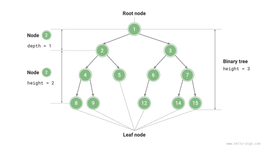
Diagram illustrating the terminology of a binary tree, showing root, parent, child, leaf, internal node, edge, path, depth, level, and height.

An illustration of key binary tree terminology.

Fundamental Components

Every node in a binary tree typically holds:

Data: The actual value or information stored within the node.
Left Child Pointer: A reference (or pointer) to the node's left child. If no left child exists, this pointer is typically null.
Right Child Pointer: A reference (or pointer) to the node's right child. If no right child exists, this pointer is also typically null.

Key Terminology

Root: The topmost node in the tree. It's the only node without a parent. A binary tree has exactly one root, unless it's empty.
Parent Node: A node that has one or more child nodes.
Child Node: A node that is directly connected to another node when moving away from the root.
Leaf Node (or External Node): A node that has no children. These are the terminal nodes of the tree.
Internal Node (or Non-Leaf Node): A node that has at least one child.
Edge: The link or connection between a parent node and its child node.
Subtree: Any node in the tree, along with all its descendants (children, grandchildren, etc.), forms a subtree. Both the left child and right child of a node are roots of their respective left and right subtrees.
Path: A sequence of nodes and edges connecting a node with a descendant.
Level of a Node: The number of edges on the path from the root node to that specific node. The root node is at level 0.
Height of a Tree: The number of edges on the longest path from the root node to any leaf node. An empty tree has a height of -1, and a tree with only a root node has a height of 0.
Depth of a Node: Similar to level, it's the number of edges from the root to the node.

The Recursive Nature of Binary Trees

A defining characteristic of binary trees is their recursive definition: A binary tree is either empty, or it consists of a root node and two disjoint binary trees called the left subtree and the right subtree. This recursive structure lends itself well to algorithms that operate on trees, as many tree operations can be defined recursively.

Exploring the Spectrum: Types of Binary Trees

Binary trees are not a one-size-fits-all structure. Various specialized types have emerged, each with unique properties catering to different computational needs. Understanding these types is key to selecting the right tree structure for a given problem.

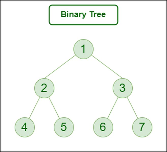
Illustration showing different types of binary trees, including full, complete, and perfect binary trees.

Visual comparison of different binary tree configurations.

Classifications Based on Structure and Node Distribution

Full Binary Tree (or Proper Binary Tree)

In a full binary tree, every node has either zero or two children. There are no nodes with only one child. This means all internal nodes have exactly two children.
Complete Binary Tree

A complete binary tree is one where all levels are completely filled, except possibly the last level. If the last level is not full, all its nodes must be as far left as possible. This property is particularly useful for array-based representations of trees, such as in heaps.
Perfect Binary Tree

A perfect binary tree is a type of full binary tree where all internal nodes have exactly two children, and all leaf nodes are at the same level (or depth). This results in a perfectly symmetrical and filled tree structure.
Balanced Binary Tree

While not a strict structural definition like the others, a balanced binary tree is one where the heights of the left and right subtrees of any node differ by at most one. This property is crucial for ensuring efficient search operations (e.g., in AVL trees or Red-Black trees), preventing the tree from becoming too skewed.
Degenerate (or Pathological) Tree

This is an extreme case where each parent node has only one child (either left or right). Such a tree essentially behaves like a linked list in terms of performance for many operations, losing the typical advantages of a tree structure.
Skewed Binary Tree

A skewed binary tree is a type of degenerate tree that is heavily dominated by either left children (left-skewed tree) or right children (right-skewed tree).
Extended Binary Tree (or 2-Tree)

An extended binary tree is formed from a regular binary tree by replacing every null subtree (empty child pointer) with a special "external" or "dummy" node. The original nodes are then considered "internal" nodes. The resulting tree is always a full binary tree.

Characteristic Properties of Binary Trees

Binary trees possess several mathematical properties that are fundamental to their analysis and application. These properties often relate the number of nodes, leaves, height, and levels of a tree.

Key Mathematical Relationships

Maximum Nodes at a Level: The maximum number of nodes at any level l (where the root is at level 0) in a binary tree is \(2^l\).
Maximum Nodes for a Given Height: The maximum number of nodes in a binary tree of height h is \(2^{h+1} - 1\). This occurs when the tree is perfect.
Minimum Height for Given Nodes: For a binary tree with n nodes, the minimum possible height is \(\lfloor \log_2 n \rfloor\). This minimum height is achieved when the tree is as balanced and compact as possible (like a complete or perfect tree).
Relationship between Leaves and Internal Nodes: In any non-empty full binary tree, if i is the number of internal nodes and l is the number of leaf nodes, then l = i + 1.
Nodes in a Perfect Binary Tree: A perfect binary tree of height h has exactly \(2^{h+1} - 1\) nodes, of which \(2^h\) are leaf nodes.

These properties are crucial for analyzing the efficiency of algorithms that operate on binary trees, particularly for operations like searching, insertion, and deletion.

Navigating and Modifying: Operations on Binary Trees

Several standard operations allow us to interact with and manipulate binary trees. The efficiency of these operations often depends on the tree's height and balance.

This video provides a deep dive into binary tree data structures, covering essential concepts for efficient data storage, searching, and sorting.

Traversal: Visiting Every Node

Traversal refers to the process of visiting each node in a tree exactly once in a systematic way. There are several common traversal methods:

Inorder Traversal (Left, Root, Right): Visits the left subtree, then the root node, and finally the right subtree. For Binary Search Trees (BSTs), an inorder traversal visits nodes in ascending order.
Preorder Traversal (Root, Left, Right): Visits the root node first, then the left subtree, and then the right subtree. Useful for creating a copy of the tree or getting prefix expressions.
Postorder Traversal (Left, Right, Root): Visits the left subtree, then the right subtree, and finally the root node. Useful for deleting nodes in a tree (as children are processed before the parent) or getting postfix expressions.
Level-Order Traversal (Breadth-First Traversal): Visits nodes level by level, from left to right at each level. This is typically implemented using a queue.

Modification Operations

Insertion: Adding a new node to the tree. The specific location of insertion depends on the type of binary tree (e.g., in a Binary Search Tree, it depends on the value; in a complete binary tree, it's the next available spot from the left).
Deletion: Removing a node from the tree. This can be complex, as it requires maintaining the tree's structural properties. The process varies significantly based on whether the node to be deleted is a leaf, has one child, or has two children.

Query Operations

Searching: Finding a specific node containing a particular value. In general binary trees, this might require traversing a significant portion of the tree. However, specialized binary trees like Binary Search Trees optimize this operation.
Finding Height/Depth: Calculating the height of the tree or the depth of a specific node.
Checking Properties: Determining if a tree is full, complete, perfect, or balanced.

Comparative Analysis of Binary Tree Types

Different types of binary trees exhibit varying characteristics in terms of balance, node distribution, and suitability for certain operations. The radar chart below provides a conceptual comparison of several binary tree types across key attributes. Note that these are general tendencies and specific implementations or scenarios might differ.

Radar chart comparing idealized characteristics of different binary tree types. "Balance" refers to height balance, "Node Fullness" to how filled the levels are, "Search Efficiency (Worst Case)" to performance in non-ideal scenarios (lower is better), "Ease of Basic Implementation" to coding complexity for core structure, and "Predictable Structure" to the regularity of node placement.

Practical Implementations: Where Binary Trees Shine

Binary trees are not just theoretical constructs; they are fundamental to many practical applications in computer science and beyond.

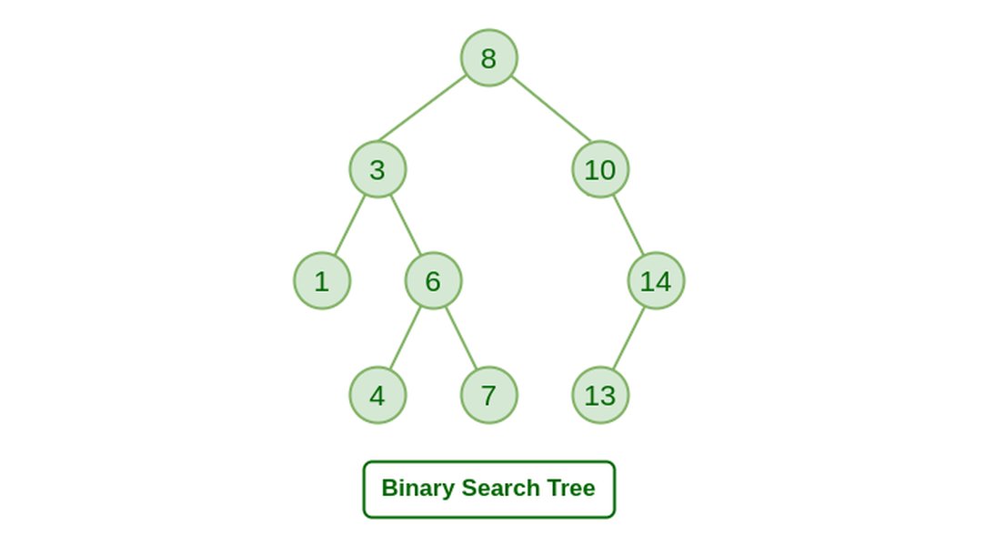
A diagram illustrating a Binary Search Tree (BST) with nodes and values, showing the ordering property.

Example of a Binary Search Tree, a common application of binary trees for efficient searching.

Binary Search Trees (BSTs): Perhaps the most well-known application. BSTs maintain a specific ordering property (left child < root < right child), allowing for efficient searching, insertion, and deletion operations, often with O(log n) average time complexity. They are used in database indexing and symbol tables in compilers.
Expression Trees: Used to represent mathematical expressions. Internal nodes are operators, and leaf nodes are operands. Traversal of an expression tree can yield prefix, infix, or postfix notations of the expression, and it's used in compilers for parsing and evaluating expressions.
Heaps (Priority Queues): Heaps are typically implemented using complete binary trees (often stored in arrays). Max-heaps and min-heaps are used to efficiently retrieve the maximum or minimum element, forming the basis of priority queues, which are essential in many algorithms (e.g., Dijkstra's, Prim's) and operating system scheduling.
Huffman Coding Trees: Used in data compression algorithms. A binary tree is constructed based on the frequency of characters in a data set, assigning shorter codes to more frequent characters.
File Systems: Hierarchical file and directory structures in operating systems can be modeled as trees (though not always strictly binary). File explorers use tree-like structures for navigation.
Document Object Model (DOM): The DOM, which represents the structure of HTML and XML documents, is a tree structure. While not strictly binary, tree concepts are fundamental, and parts might be processed or represented internally using binary tree principles.
Routing Algorithms: In computer networks, trees (including binary trees or structures derived from them like tries) can be used in routing tables to determine efficient paths for data packets.
Decision Trees: In machine learning and artificial intelligence, decision trees are used for classification and regression. Each internal node represents a "test" on an attribute, each branch represents the outcome of the test, and each leaf node represents a class label or a decision.
Game Trees: In AI for games (e.g., chess, tic-tac-toe), game trees represent all possible moves from a current state. Binary trees can be a part of this, especially in simpler games or specific decision points.
Cladograms in Biology: Used to represent evolutionary relationships between different species, where branching points indicate common ancestors.

Visualizing Binary Tree Concepts: A Mindmap

The mindmap below provides a hierarchical overview of the core concepts related to binary trees, branching from the central idea to its types, properties, operations, and common applications. This visual representation helps to connect the various aspects discussed.

mindmap root["Binary Tree Fundamentals"] id1["Definition
Each node has at most two children (left & right)"] id2["Key Terminology"] id2_1["Root"] id2_2["Node"] id2_3["Edge"] id2_4["Leaf"] id2_5["Internal Node"] id2_6["Parent/Child"] id2_7["Subtree"] id2_8["Height/Depth/Level"] id3["Types of Binary Trees"] id3_1["Full Binary Tree
(0 or 2 children)"] id3_2["Complete Binary Tree
(Levels filled, last level left-aligned)"] id3_3["Perfect Binary Tree
(All levels full, leaves at same depth)"] id3_4["Balanced Binary Tree
(Subtree heights differ by at most 1)"] id3_5["Degenerate/Pathological Tree
(Linked list-like)"] id3_6["Skewed Tree (Left/Right)"] id4["Core Properties"] id4_1["Max nodes at level L = 2^L"] id4_2["Max nodes for height H = 2^(H+1) - 1"] id4_3["Recursive structure"] id5["Common Operations"] id5_1["Traversal"] id5_1_1["Inorder (LNR)"] id5_1_2["Preorder (NLR)"] id5_1_3["Postorder (LRN)"] id5_1_4["Level-order"] id5_2["Insertion"] id5_3["Deletion"] id5_4["Search"] id6["Applications"] id6_1["Binary Search Trees (BSTs)"] id6_2["Expression Trees"] id6_3["Heaps (Priority Queues)"] id6_4["Huffman Coding"] id6_5["File Systems"] id6_6["DOM Representation"] id6_7["Decision Trees (AI)"]

Mindmap illustrating the interconnected concepts of binary trees.

Comparing Binary Tree Traversal Methods

Traversal is a fundamental operation on binary trees, involving visiting each node in a specific sequence. The choice of traversal method depends on the task at hand. The table below summarizes the key characteristics of common traversal techniques.

Traversal Type	Order of Visit (N=Node, L=Left, R=Right)	Primary Use Case	Recursive Nature
Inorder Traversal	LNR (Left Subtree, Node, Right Subtree)	Retrieving data in sorted order from a Binary Search Tree (BST).	Naturally recursive; can be implemented iteratively using a stack.
Preorder Traversal	NLR (Node, Left Subtree, Right Subtree)	Creating a copy of the tree (prefix notation of expression trees). Exploring roots before leaves.	Naturally recursive; can be implemented iteratively using a stack.
Postorder Traversal	LRN (Left Subtree, Right Subtree, Node)	Deleting nodes from a tree (processing children before parent), postfix notation of expression trees.	Naturally recursive; can be implemented iteratively using two stacks or modified preorder.
Level-Order Traversal (Breadth-First)	Visits nodes level by level, from top to bottom, and left to right within each level.	Finding the shortest path between two nodes in terms of levels. Useful when order of processing by depth is important.	Typically implemented iteratively using a queue. Not as naturally recursive as depth-first traversals.

References

Last updated May 6, 2025