Unlock the Power of Density: How DBSCAN Finds Hidden Patterns in Your Data

Discover the intuitive algorithm that clusters data based on closeness, identifies outliers, and doesn't need you to guess the number of groups.

Key Insights into DBSCAN

Shape Agnostic Clustering: Unlike algorithms like K-Means, DBSCAN excels at finding clusters of arbitrary shapes, not just spherical ones.
Automatic Outlier Detection: It naturally identifies points in low-density regions as noise or outliers, making it robust for real-world, messy data.
No Predefined Cluster Count: You don't need to specify the number of clusters beforehand; DBSCAN determines them based on the data's density structure.

Understanding DBSCAN: Clustering by Density

DBSCAN, which stands for Density-Based Spatial Clustering of Applications with Noise, is a highly regarded clustering algorithm first introduced in 1996 by Martin Ester, Hans-Peter Kriegel, Jörg Sander, and Xiaowei Xu. Its significance in the field was recognized with the Test of Time Award at the ACM SIGKDD conference in 2014. Unlike partitioning methods (like K-Means) or hierarchical methods, DBSCAN groups data points based on their density, allowing it to discover clusters of complex shapes and effectively handle noise.

The core idea is that a cluster is a dense region of points separated from other dense regions by areas of lower point density. Points that don't belong to any dense region are classified as noise or outliers.

The Building Blocks: Key Parameters

DBSCAN's behavior is primarily controlled by two crucial parameters:

Epsilon (\( \epsilon \)): This defines the radius of the neighborhood around a data point. Any point within this distance is considered a neighbor. Choosing the right \( \epsilon \) is critical; too small, and dense areas might be fragmented; too large, and distinct clusters might merge.
MinPts (Minimum Points): This specifies the minimum number of data points (including the point itself) required within a point's \( \epsilon \)-neighborhood for it to be considered part of a dense region (a core point). A common heuristic is to set MinPts >= D+1, where D is the dimensionality of the data, though MinPts=3 is often a good starting point for 2D data.

Classifying Data Points

Based on the \( \epsilon \) and MinPts parameters, DBSCAN classifies each point in the dataset into one of three types:

Core Point: A point is a core point if its \( \epsilon \)-neighborhood contains at least MinPts points (including itself). These points are located in the interior of a dense cluster.
Border Point: A point is a border point if it is not a core point (i.e., it has fewer than MinPts neighbors within \( \epsilon \)), but it falls within the \( \epsilon \)-neighborhood of at least one core point. Border points lie on the edge of a cluster.
Noise Point (Outlier): A point is classified as noise if it is neither a core point nor a border point. These points reside in low-density regions and do not belong to any cluster.

The DBSCAN Clustering Process: Step-by-Step

The algorithm systematically explores the dataset to identify density-connected regions:

Initialization: Start with an arbitrary, unvisited data point.
Neighborhood Check: Determine the point's \( \epsilon \)-neighborhood. Count the number of points within this radius.
Point Classification:
- If the neighborhood contains fewer than MinPts points, initially mark the point as noise. It might later be reclassified as a border point if it's found to be in the neighborhood of a core point.
- If the neighborhood contains MinPts or more points, mark the point as a core point and start a new cluster.
Cluster Expansion:
- Add the core point to the current cluster.
- Find all density-reachable points from this core point. This involves iteratively finding all points within the \( \epsilon \)-neighborhood of the core point and any newly added core points.
- If a reachable point is also a core point, expand the cluster further from it.
- If a reachable point is a border point (not a core point itself), add it to the cluster but do not expand further from it.
- If a point initially marked as noise is found within the \( \epsilon \)-neighborhood of a core point during expansion, reclassify it as a border point and add it to the cluster.
Iteration: Repeat steps 1-4 for all unvisited points in the dataset.
Completion: Once all points have been visited and classified (as core, border, or noise) and assigned to a cluster (or marked as noise), the algorithm terminates.

Visualizing DBSCAN Concepts

This mindmap provides a hierarchical overview of the DBSCAN algorithm, breaking down its core components, process, characteristics, and common uses.

mindmap root["DBSCAN Algorithm"] ["Core Concepts"] ["Epsilon (ε)"] ["Neighborhood radius"] ["MinPts"] ["Minimum points for density"] ["Point Types"] ["Core Point"] ["Border Point"] ["Noise Point (Outlier)"] ["Clustering Process"] ["Start with arbitrary point"] ["Check ε-neighborhood"] ["Classify (Core/Border/Noise)"] ["Expand cluster from Core Points"] ["Iterate until all points visited"] ["Advantages"] ["Handles arbitrary shapes"] ["No need to pre-specify cluster count"] ["Robust to outliers/noise"] ["Disadvantages"] ["Sensitive to parameters (ε, MinPts)"] ["Struggles with varying densities"] ["Potential high computational cost"] ["'Curse of dimensionality' issues"] ["Applications"] ["Geographic Information Systems (GIS)"] ["Anomaly Detection (Fraud, Network Traffic)"] ["Image Segmentation"] ["Market Segmentation"] ["Bioinformatics"]

Why Choose DBSCAN? Advantages and Disadvantages

Strengths of DBSCAN

Finds Arbitrarily Shaped Clusters: Unlike K-Means which assumes spherical clusters, DBSCAN can identify clusters of various shapes (e.g., linear, concave) based on density connectivity.
No Need to Specify Cluster Count: The algorithm automatically determines the number of clusters based on the data distribution and parameters, eliminating guesswork.
Robust Outlier Handling: It has a built-in mechanism to identify and isolate noise points, making it suitable for datasets containing outliers that could skew other algorithms.
Conceptually Intuitive: The density-based approach often aligns well with human intuition about what constitutes a cluster.

Limitations of DBSCAN

Parameter Sensitivity: The quality of the clustering results heavily depends on the choice of \( \epsilon \) and MinPts. Finding optimal values can be challenging and may require domain knowledge or experimentation (e.g., using k-distance plots).
Difficulty with Varying Densities: DBSCAN struggles when clusters have significantly different densities, as a single set of \( \epsilon \) and MinPts may not be appropriate for all clusters. Some dense clusters might merge, or sparser clusters might be missed or broken up.
High-Dimensional Data Issues: In very high-dimensional spaces (the "curse of dimensionality"), the concept of density becomes less meaningful as points tend to be sparse and equidistant, making \( \epsilon \) selection difficult.
Computational Cost: The naive implementation has a time complexity of O(n²). While spatial indexing can improve this to O(n log n) on average, performance can degrade on degenerate or highly clustered data.
Memory Complexity (Scikit-learn): The popular scikit-learn implementation pre-computes neighborhood queries, which can lead to high memory usage (O(n*d), where d is the average number of neighbors) for large datasets, deviating from the original algorithm's O(n) memory complexity.
Non-Deterministic Border Points: A border point might be reachable from core points of multiple clusters. Depending on the order of processing, it might be assigned to either cluster, leading to slight variations in results.
Doesn't Predict New Points: DBSCAN is a non-parametric model and doesn't inherently provide a way to assign new, unseen data points to existing clusters without re-running the algorithm or using extensions.

DBSCAN Performance Characteristics

The radar chart below offers a visual comparison of DBSCAN's key performance aspects. Higher values indicate stronger performance in that category. Note that these are qualitative assessments based on the algorithm's design.

This chart highlights DBSCAN's strengths in handling complex shapes and outliers, and its independence from predefined cluster counts. However, it also shows its challenges with parameter tuning, varying densities, scalability (especially memory in some implementations), and high-dimensional data.

Parameter Tuning: The Art of \( \epsilon \) and MinPts

Selecting appropriate values for \( \epsilon \) and MinPts is crucial for successful DBSCAN clustering. It often involves some experimentation and understanding of the data.

Choosing MinPts

A common rule of thumb is `MinPts >= Dimensionality + 1`.
For 2D data, `MinPts = 3` or `MinPts = 4` is often a good starting point.
Higher values of MinPts generally lead to denser clusters being identified and more points being classified as noise. It makes the algorithm less sensitive to outliers but might miss smaller clusters.

Choosing Epsilon (\( \epsilon \))

This is often more challenging than choosing MinPts.
One popular technique involves plotting a k-distance graph. For a chosen `k` (often `k = MinPts - 1`), calculate the distance to the k-th nearest neighbor for every point. Sort these distances in ascending order and plot them.
The graph typically shows a "knee" or "elbow" point. The distance value at this elbow is often a good candidate for \( \epsilon \). This point represents a threshold where distances start increasing significantly, suggesting a transition from dense regions to sparser regions.
If \( \epsilon \) is too small, a large part of the data might be classified as noise.
If \( \epsilon \) is too large, distinct clusters might merge into one, or the majority of points might form a single large cluster.

Parameter Impact Summary

The following table summarizes the general effects of adjusting \( \epsilon \) and MinPts:

Parameter Change	Effect on Clusters	Effect on Noise
Increase \( \epsilon \)	Fewer, larger clusters (potential merging)	Less noise
Decrease \( \epsilon \)	More, smaller clusters (potential fragmentation)	More noise
Increase MinPts	Requires denser regions; fewer clusters formed	More noise
Decrease MinPts	Allows sparser regions; more clusters formed	Less noise

Visualizing DBSCAN in Action

The following images illustrate how DBSCAN identifies clusters and noise points in different datasets. Notice how it effectively handles non-spherical shapes and separates outliers.

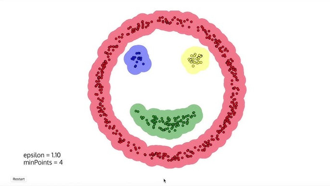
These visuals demonstrate DBSCAN's ability to group points based on density connectivity, leading to the discovery of clusters that other algorithms might miss, while correctly labeling isolated points as noise.

Learn More: DBSCAN Explained Visually

For a deeper dive into the mechanics of DBSCAN, including how core points, border points, and noise are identified step-by-step, watch this explanatory video:

This video provides a clear, simple explanation of the DBSCAN algorithm's core logic and how it processes data points to form clusters based on density, making the concepts easier to grasp.

Applications: Where is DBSCAN Used?

DBSCAN's unique capabilities make it suitable for a wide range of applications across various domains:

Geographic Information Systems (GIS): Identifying areas of similar land use in satellite imagery, clustering points of interest (e.g., crime hotspots, disease outbreaks), grouping locations with similar activities.
Anomaly Detection: Detecting unusual patterns or outliers in financial transactions (fraud detection), network traffic analysis (intrusion detection), or sensor readings.
Image Analysis & Computer Vision: Segmenting images based on pixel density or color, detecting shapes and patterns.
Market Segmentation & Customer Analytics: Grouping customers with similar purchasing behaviors or demographic profiles, identifying distinct market segments.
Bioinformatics: Clustering gene expression data or protein structures.
Recommendation Systems: Grouping users or items with similar preferences.

Implementation and Variations

DBSCAN is readily available in popular machine learning libraries, such as scikit-learn in Python, making it easy to apply to datasets. While powerful, researchers have developed extensions to address some of its limitations:

OPTICS (Ordering Points To Identify the Clustering Structure): An algorithm that addresses the varying density issue by creating an augmented ordering of the database representing its density-based clustering structure. It avoids the need for a single global \( \epsilon \) value.
HDBSCAN (Hierarchical DBSCAN): Extends DBSCAN by converting it into a hierarchical clustering algorithm, making it more robust to parameter selection and capable of finding clusters of varying densities.

Frequently Asked Questions (FAQ)

What does DBSCAN stand for? ▼

DBSCAN stands for Density-Based Spatial Clustering of Applications with Noise. The name highlights its core mechanism (density), its origin in spatial databases, and its ability to handle noisy data.

How is DBSCAN different from K-Means? ▼

Key differences include:

Cluster Shape: K-Means assumes clusters are spherical and assigns points to the nearest centroid. DBSCAN finds arbitrarily shaped clusters based on density.
Number of Clusters: K-Means requires the number of clusters (k) to be specified beforehand. DBSCAN determines the number of clusters automatically.
Outliers: K-Means forces every point into a cluster. DBSCAN explicitly identifies and labels outliers (noise points).
Approach: K-Means is a centroid-based partitioning algorithm. DBSCAN is a density-based algorithm.

How do I choose the parameters \( \epsilon \) and MinPts? ▼

Choosing parameters often requires experimentation:

MinPts: Often set based on data dimensionality (e.g., MinPts >= D+1) or domain knowledge. Higher values lead to denser clusters. Start with values like 3 or 4 for 2D data.
Epsilon (\( \epsilon \)): Can be estimated using a k-distance graph. Plot the distance to the k-th nearest neighbor (where k = MinPts-1) for all points, sorted by distance. Look for the "elbow" or "knee" in the plot, which indicates a suitable \( \epsilon \) value.

Visual inspection of results with different parameter combinations is also common.

What are the main limitations of DBSCAN? ▼

The main limitations include:

Sensitivity to the \( \epsilon \) and MinPts parameters.
Difficulty handling clusters with widely varying densities simultaneously.
Performance challenges with very high-dimensional data (curse of dimensionality).
Potential high computational cost (O(n²)) without spatial indexing, or high memory usage in some implementations like scikit-learn.