
Differential Equations for Electric Circuits
Unraveling the Mathematical Foundations of Circuit Behavior
Key Takeaways
- Essential Modeling Tool: Differential equations are fundamental in predicting and analyzing the dynamic behavior of electric circuits involving resistors, inductors, and capacitors.
- Kirchhoff’s Laws: These laws are the cornerstone for formulating the differential equations that govern circuit dynamics.
- Diverse Solution Methods: Techniques such as separation of variables, integrating factors, and Laplace transforms are crucial for solving these equations and understanding circuit responses.
Introduction to Differential Equations in Electric Circuits
Differential equations are indispensable in the field of electrical engineering for modeling and analyzing the behavior of electric circuits. By describing the relationships between voltage, current, and time, these equations provide insights into how circuits respond to various inputs and conditions. Whether dealing with simple circuits composed of a single resistor and capacitor or complex networks involving multiple inductors and capacitors, differential equations offer a mathematical framework to predict circuit performance and guide design decisions.
Fundamental Components and Their Mathematical Relationships
Resistors (R)
Resistors impede the flow of electric current, adhering to Ohm's Law: \[ V = IR \] where \( V \) is the voltage across the resistor, \( I \) is the current through it, and \( R \) is the resistance value. This linear relationship forms the basis for analyzing circuits with resistive elements.
Inductors (L)
Inductors store energy in a magnetic field when current flows through them. Their voltage-current relationship is governed by: \[ V = L \frac{dI}{dt} \] where \( L \) is the inductance and \( \frac{dI}{dt} \) is the rate of change of current. This relationship introduces a differential component to circuit equations.
Capacitors (C)
Capacitors store energy in an electric field, with their current-voltage relationship given by: \[ I = C \frac{dV}{dt} \] where \( C \) is the capacitance and \( \frac{dV}{dt} \) is the rate of change of voltage across the capacitor. This adds another layer of differential complexity to circuit analysis.
Kirchhoff’s Laws: Foundations for Circuit Equations
Kirchhoff's Voltage Law (KVL)
KVL states that the sum of all electrical potential differences around any closed loop in a circuit equals zero: \[ \sum V = 0 \] This law ensures energy conservation within the circuit and is pivotal in formulating differential equations for circuit loops.
Kirchhoff's Current Law (KCL)
KCL asserts that the total current entering a junction equals the total current leaving the junction: \[ \sum I_{in} = \sum I_{out} \] This principle is essential for analyzing complex networks where multiple currents intersect.
Types of Electric Circuits and Their Governing Differential Equations
Series RL Circuit
A series RL circuit consists of a resistor and an inductor connected in series with a voltage source. Applying KVL yields the first-order linear differential equation: \[ V(t) = IR + L \frac{dI}{dt} \] Rearranging terms: \[ L \frac{dI}{dt} + RI = V(t) \] This equation describes how the current \( I(t) \) evolves over time in response to the applied voltage.
Series RC Circuit
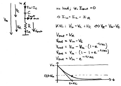
In a series RC circuit, a resistor and a capacitor are connected in series with a voltage source. Applying KVL leads to: \[ V(t) = IR + \frac{1}{C} \int I \, dt \] Differentiating both sides with respect to time: \[ RC \frac{dV_C}{dt} + V_C = V_s(t) \] where \( V_C \) is the voltage across the capacitor and \( V_s(t) \) is the source voltage. This first-order differential equation models the charging and discharging behavior of the capacitor.
Series RLC Circuit
A series RLC circuit includes a resistor, inductor, and capacitor connected in series with a voltage source. Applying KVL results in a second-order linear differential equation: \[ V(t) = IR + L \frac{dI}{dt} + \frac{1}{C} \int I \, dt \] Differentiating and rearranging: \[ L C \frac{d^2V_C}{dt^2} + R C \frac{dV_C}{dt} + V_C = V_s(t) \] This equation facilitates the analysis of oscillatory behaviors and damping effects within the circuit.
Parallel and Series-Parallel Circuits
More complex configurations, such as parallel and series-parallel circuits, involve multiple resistors, inductors, and capacitors. Applying Kirchhoff's laws in these circuits leads to systems of differential equations that account for various currents and voltages. Techniques like substitution and integration are often employed to solve these equations, providing a comprehensive understanding of the circuit's dynamic responses.
Solution Techniques for Circuit Differential Equations
Separation of Variables
This method involves rearranging the differential equation to isolate the dependent and independent variables on opposite sides. It is particularly useful for first-order linear differential equations, such as those found in RL and RC circuits. The technique simplifies the equation, making it easier to integrate and solve for the desired variable.
Integrating Factor Method
Applicable to first-order linear differential equations, the integrating factor method transforms the equation into an exact differential, facilitating straightforward integration. For instance, in a series RL circuit, multiplying both sides by \( e^{\frac{R}{L}t} \) allows the equation to be integrated, yielding the current as a function of time: \[ I(t) = \frac{V}{R} \left(1 - e^{-\frac{R}{L} t}\right) \] This solution illustrates how the current asymptotically approaches its steady-state value over time ([4]).
Laplace Transforms
Laplace transforms convert differential equations into algebraic equations in the \( s \)-domain, simplifying the process of solving complex circuits with initial conditions. After solving the transformed equation, the inverse Laplace transform is applied to return to the time domain. This method is especially effective for handling second-order circuits like RLC configurations, where oscillatory and damping behaviors are prominent ([5]).
Homogeneous and Particular Solutions
The complete solution to a non-homogeneous differential equation consists of two parts:
- Homogeneous Solution: Solves the associated homogeneous equation (\( V_s(t) = 0 \)), representing the natural response of the circuit.
- Particular Solution: Accounts for the external input or forcing function (\( V_s(t) \)), representing the forced response.
Applications of Differential Equations in Electric Circuit Analysis
Transient Analysis
Transient analysis examines how circuits respond to changes over time, such as the charging of a capacitor or the current decay in an inductor. Differential equations enable the prediction of these transient states, providing critical information for designing circuits that behave reliably during startup or switching events.
Steady-State Analysis and Time Constants
Steady-state analysis focuses on the long-term behavior of circuits after transients have settled. Time constants, represented by \( \tau = RC \) for RC circuits and \( \tau = \frac{L}{R} \) for RL circuits, quantify the rate at which circuits approach their steady-state values. Differential equations facilitate the calculation of these time constants, essential for timing applications and filtering responses.
AC Circuit Analysis
In alternating current (AC) circuits, differential equations describe the sinusoidal inputs and the resulting sinusoidal steady-state responses. Analyzing these circuits involves solving differential equations with sinusoidal forcing functions, allowing engineers to design circuits with desired frequency responses and impedance characteristics.
Predictive Circuit Design
By solving differential equations, engineers can predict how circuits will behave under various conditions, leading to more efficient and reliable designs. This predictive capability is crucial for developing technologies ranging from simple consumer electronics to complex communication systems ([7]).
Example Problems and Solutions
Example 1: Series RL Circuit
Consider a series RL circuit with \( R = 10 \, \Omega \), \( L = 0.5 \, H \), and an applied voltage \( V(t) = 10 \, V \). The governing differential equation is: \[ 0.5 \frac{dI}{dt} + 10I = 10 \] Using the integrating factor method, the solution is: \[ I(t) = 1 \left(1 - e^{-\frac{10}{0.5} t}\right) = 1 \left(1 - e^{-20t}\right) \] This solution indicates that the current gradually approaches 1 A as time progresses, with a rapid rise due to the high time constant (\( \tau = \frac{L}{R} = 0.05 \, s \)).
Example 2: Series RLC Circuit
In a series RLC circuit with \( R = 1 \, \Omega \), \( L = 0.2 \, H \), \( C = 0.01 \, F \), and an applied voltage \( V(t) = \sin(5t) \), the differential equation becomes: \[ 0.2 \frac{d^2q}{dt^2} + \frac{dq}{dt} + 100q = \sin(5t) \] Solving this equation involves finding both the homogeneous and particular solutions. The homogeneous solution captures the natural oscillations and damping, while the particular solution aligns with the sinusoidal input. The total charge \( q(t) \) can then be differentiated to find the current \( I(t) \), revealing the circuit's response to the AC input.
Educational Resources and Further Reading
Comprehensive Course Materials
- Johns Hopkins University Course Notes on Linear Circuit Theory
- Math Tutor DVD: Applications of Differential Equations in Circuits
Interactive Tutorials and Examples
- Interactive Examples of RL Circuits
- Application of Laplace Transform to Circuits
- RLC Circuit Differential Equations
Foundational Modeling Examples
Conclusion
Differential equations serve as the mathematical backbone for understanding and predicting the behavior of electric circuits. By leveraging Kirchhoff's laws and the inherent properties of resistors, inductors, and capacitors, these equations enable engineers to model complex circuit dynamics, analyze transient and steady-state responses, and design systems with precise performance characteristics. Mastery of differential equation techniques, including separation of variables, integrating factors, and Laplace transforms, is essential for advancing in electrical engineering and fostering innovation in circuit design and analysis.
Last updated January 10, 2025