
Unlocking Economic Stability: Understanding Equilibrium in Consumption and Wealth
Explore steady-state and cointegration relationships, their testing methods, and profound implications for the consumption-wealth dynamic.
Highlights
- Equilibrium Defined: Equilibrium relationships signify a state of balance where economic variables, like consumption and wealth, achieve stability over time, either remaining constant (steady-state) or moving together predictably in the long run (cointegration).
- Consumption & Wealth Link: Economic theories propose a long-term equilibrium relationship between consumption and total wealth (comprising asset wealth and the present value of labor income), often confirmed empirically through cointegration analysis.
- Critical Implications: Identifying an equilibrium relationship (especially cointegration) suggests long-run predictability, temporary deviations, and significant insights for understanding the wealth effect, guiding economic policy, and improving forecasting.
Defining Equilibrium Relationships
The Concept of Balance in Systems
At its core, an equilibrium relationship describes a state of balance within a system where opposing forces counteract each other, leading to a stable condition. In economic or physical contexts, this means that variables have reached a point where they either cease to change significantly over time or their movements are interconnected in a predictable, long-term manner. It's a condition where inputs and outputs might balance, preventing further net changes in key variables, even if underlying processes continue.
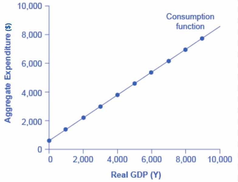
An illustration of equilibrium in the context of aggregate expenditure.
Two Key Types: Steady-State vs. Cointegration
While the general concept is balance, equilibrium manifests in different ways. Two fundamental types relevant to dynamic systems, particularly in economics, are steady-state equilibrium and cointegration relationships:
- Steady-State Equilibrium: Characterized by variables remaining constant or growing at a constant, stable rate over time. It represents a specific type of long-run balance where the system settles into an unchanging state or a balanced growth path.
- Cointegration Relationship: A statistical concept describing a long-run equilibrium connection between two or more time series variables that are individually non-stationary (meaning they tend to drift over time without returning to a fixed mean) but move together in such a way that a linear combination of them *is* stationary.
Understanding the distinction between these two forms of equilibrium is crucial for analyzing economic relationships like the one between consumption and wealth.
Steady-State Equilibrium Explained
What is Steady State?
A steady-state equilibrium signifies a condition where the essential variables within a dynamic system remain constant over time, or grow at a constant rate, because inflows and outflows are perfectly balanced. Despite ongoing processes within the system, the overall state appears stable and unchanging.
Examples Across Disciplines:
- Physical Systems: In thermal conductivity tests, a steady state is reached when heat flow and temperature differences across a sample stabilize. Similarly, in fluid dynamics, it involves achieving a stable flow rate.
- Chemical Kinetics: The "steady-state approximation" assumes the concentration of reactive intermediates remains constant because their rate of formation equals their rate of consumption, simplifying the analysis of reaction mechanisms.
- Economics: In economic growth models (like the Solow model), the steady state refers to a long-run condition where variables like capital per worker and output per worker are constant or grow at a constant rate. It can represent a theoretical long-run balance where consumption-to-wealth ratios might stabilize under specific model assumptions.
Testing for Steady State
Identifying a steady state involves confirming the stability or constant growth rate of key variables:
- Observation in Experiments: In physical or chemical systems, researchers hold control variables constant and monitor response variables until they stabilize, confirming the steady state empirically.
- Model Analysis: Economic models can be solved for their steady-state conditions, predicting the long-run levels or growth rates variables will converge to under specific assumptions (e.g., the Solow Growth Model).
- Time Series Analysis: Statistical tests, such as unit root tests (like the Augmented Dickey-Fuller test), can assess whether economic time series data are stationary (fluctuating around a constant mean) or exhibit a constant trend, which can be indicative of steady-state behavior in certain contexts.
Cointegration Relationships Unveiled
Beyond Constant States: Long-Run Connections
Cointegration offers a framework for understanding equilibrium relationships between variables that are themselves changing over time, often in a non-stationary manner (exhibiting trends or random walks). If two or more non-stationary time series are cointegrated, it means they share a common underlying stochastic trend and are linked by a long-run equilibrium relationship.
Even though individual variables like consumption and wealth might drift upwards over time and experience short-term fluctuations independently, cointegration implies they cannot wander arbitrarily far from each other in the long run. There's an economic force that pulls them back towards their equilibrium relationship. The difference, or a specific linear combination, between these variables is stationary (mean-reverting).
Testing for Cointegration
Since cointegration is a statistical property, it is tested using econometric techniques on time series data:
- Pre-testing for Unit Roots: The first step is usually to test individual time series (e.g., consumption, wealth) for non-stationarity using unit root tests. Cointegration applies specifically to non-stationary variables (typically integrated of order one, I(1)).
- Engle-Granger Two-Step Method: This involves regressing one non-stationary variable on the other(s) and then testing the residuals (the differences between actual and predicted values) from this regression for stationarity. If the residuals are stationary, the variables are cointegrated.
- Johansen Test: A more robust, multivariate approach suitable when dealing with more than two variables. It can identify the number of distinct cointegrating relationships (the cointegrating rank) among a group of variables using a Vector Autoregression (VAR) framework.
- Error Correction Models (ECMs): If cointegration is confirmed, an ECM can be estimated. ECMs explicitly model both the short-run dynamics and the long-run equilibrium relationship, showing how deviations from the long-run equilibrium are "corrected" in subsequent periods. The coefficient on the error correction term indicates the speed of adjustment back to equilibrium.
Connecting Equilibrium to Consumption and Wealth
The Theoretical Link
The relationship between consumption and wealth is a cornerstone of macroeconomic theory. Foundational concepts like the Life-Cycle Hypothesis and the Permanent Income Hypothesis posit that rational individuals base their consumption decisions not just on current income, but on their expected lifetime resources, or total wealth.
Defining Wealth
In this context, "wealth" is broadly defined to encompass all resources available to support consumption over a lifetime. It typically includes:
- Asset Wealth: Tangible assets like real estate and financial assets such as stocks, bonds, and savings accounts.
- Labor Income (Human Wealth): The present value of expected future earnings from labor. This represents the economic value of an individual's skills and potential to earn income over their working life.
Therefore, the total wealth considered is \( W_t = A_t + H_t \), where \( A_t \) is asset wealth and \( H_t \) is human wealth (often proxied by expected labor income streams).
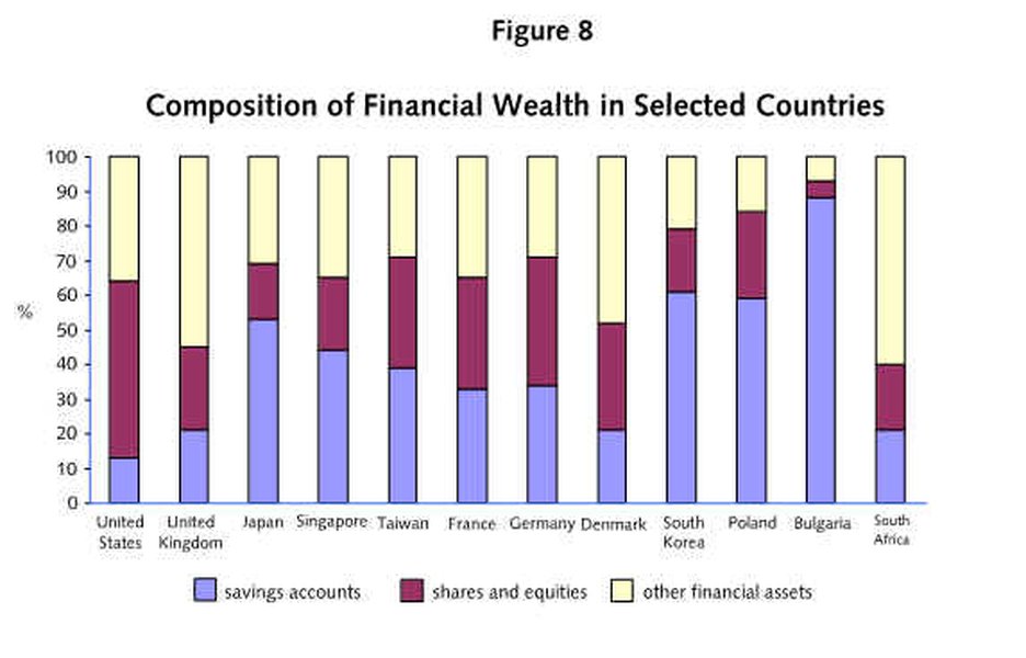
Composition of household wealth varies, encompassing financial and non-financial assets.
Empirical Evidence: Are Consumption and Wealth Cointegrated?
Given the theoretical link, economists frequently investigate whether consumption and total wealth exhibit a stable long-run relationship using time series data. Many empirical studies, often using cointegration techniques, find evidence supporting such a relationship. For instance, research suggests that aggregate consumption, asset wealth, and labor income (or proxies for it) often appear to be cointegrated.
This finding implies that, despite short-term deviations caused by economic shocks or temporary factors, consumption tends to adjust over the long run to remain proportional to total wealth. The aggregate budget constraint implies such a relationship should hold over the long term. However, the exact nature and stability of this relationship can be complex, potentially influenced by factors like wealth distribution, the type of economic shocks, and whether shocks are anticipated or unanticipated.
Visualizing the Dynamics: Consumption vs. Wealth Factors
The relationship between consumption and wealth is influenced by numerous factors, and their potential equilibrium is a dynamic interplay. The mindmap below illustrates some key components and influencing factors:
This mindmap highlights that both consumption and wealth are complex variables influenced by multiple factors. The equilibrium relationship, whether viewed as a steady state or cointegration, connects these two sides, suggesting that changes in wealth components (like stock market booms or shifts in labor income expectations) will eventually feed through to consumption patterns, and vice versa, as the system seeks balance.
Gauging the Interplay: Factors Influencing the Equilibrium Type
Whether a steady-state or cointegration framework is more appropriate for analyzing the consumption-wealth relationship depends on the context, data characteristics, and analytical goals. The radar chart below provides a conceptual comparison based on several factors:
This chart visually suggests that:
- Steady-State concepts are often more relevant for theoretical modeling, long-term growth analysis, situations assuming stability, and simpler model frameworks.
- Cointegration is particularly powerful for analyzing empirical time series data, understanding adjustments to persistent shocks, handling more complex dynamic models, and informing policies related to both short-term fluctuations and long-term trends.
For analyzing the actual historical relationship between consumption and wealth using economic data, cointegration analysis is typically the more utilized and appropriate framework due to the inherent non-stationarity and dynamic nature of these variables.
Interpreting the Implications: Why Equilibrium Matters
Identifying an equilibrium relationship between consumption and wealth, whether steady-state or cointegration, carries significant implications for economic understanding and policymaking.
Implications of a Steady-State Relationship
If consumption and wealth were found to adhere to a strict steady-state equilibrium (in levels or growth rates):
- Predictable Long Run: It implies a highly predictable long-run path where the ratio of consumption to wealth remains constant or follows a stable trajectory.
- Model Simplification: Useful for simplified theoretical models aiming to understand fundamental long-run economic forces, abstracting from short-term dynamics.
- Limited Dynamics: May not adequately capture the economy's response to shocks or the complexities of short-to-medium term adjustments.
Implications of a Cointegration Relationship
Finding cointegration between consumption and wealth is generally considered more empirically relevant and yields richer insights:
Long-Run Stability and Predictability
Cointegration confirms a stable, non-spurious long-term link. It means that despite short-term volatility, consumption and wealth do not drift apart indefinitely. This provides a basis for long-run forecasting: knowing the trajectory of wealth can help predict the long-run path of consumption, and vice versa.
The Error Correction Mechanism
A key implication is the existence of an error correction mechanism. When shocks temporarily push consumption and wealth away from their long-run equilibrium path, economic forces (like adjustments in spending or saving behavior) act to restore the relationship. The speed of this adjustment can be estimated, providing insights into how quickly the system returns to balance after a disturbance.
Understanding the Wealth Effect
Cointegration provides a robust framework for interpreting the "wealth effect" – the impact of changes in wealth on consumption. It suggests that changes in wealth (both asset and human wealth) tend to have persistent, long-lasting effects on consumption, rather than being purely transitory. However, interpreting the magnitude can be complex, as both consumption and wealth respond endogenously to underlying economic shocks. The relationship observed might reflect how both variables react to common factors (like changes in interest rates or productivity) rather than a simple causal link from wealth to consumption.
Policy and Forecasting Significance
Understanding this cointegrating link is vital for policymakers. Policies affecting wealth (e.g., monetary policy impacting asset prices, fiscal policy affecting disposable income and savings, education policies affecting human capital) can be expected to have predictable long-term consequences for consumption spending. It helps distinguish between temporary fluctuations and permanent shifts in economic trends, improving the accuracy of economic forecasts and the design of stabilization policies.
This video discusses related concepts of equilibrium income, consumption, and savings, providing context for how these macroeconomic variables interact.
Comparing the Equilibrium Concepts
The following table summarizes the key differences between steady-state and cointegration relationships in the context of consumption and wealth:
| Feature | Steady-State Equilibrium | Cointegration Relationship |
|---|---|---|
| Definition | Variables are constant or grow at a constant rate; system is unchanging or in balanced growth. | Non-stationary variables share a common trend; a linear combination is stationary; long-run link. |
| Variable Behavior | Levels or growth rates are stable and constant over the long run. | Individual variables can trend/drift over time, but do not deviate from each other indefinitely. |
| Testing Methods | Model analysis, observation of stability, unit root tests for stationarity/trend-stationarity. | Unit root pre-tests, Engle-Granger test, Johansen test, ECM estimation. |
| Typical Application Context | Theoretical growth models, long-run benchmarks, physical/chemical systems. | Empirical time series analysis, macroeconomics (consumption, income, wealth), finance. |
| Implication for C-W Link | Suggests a constant C/W ratio or balanced growth in the very long run under specific assumptions. | Implies a stable long-run relationship despite short-term fluctuations; deviations are corrected; supports persistent wealth effects. |
Frequently Asked Questions (FAQ)
What's the difference between chemical equilibrium and steady state?
Chemical equilibrium is a specific state where the rates of the forward and reverse reactions are equal, resulting in no net change in the concentrations of reactants and products. It's a closed system state. A steady state, often applied in open systems or reaction kinetics, means the concentration of certain components (like intermediates) remains constant because their rate of formation equals their rate of consumption, even if the overall reaction is proceeding and materials are flowing through the system. Steady state doesn't require the forward and reverse rates to be equal, only that the net change of the specific component is zero.
Why is cointegration so important in economics?
Many economic variables (like GDP, consumption, wealth, prices) tend to trend upwards over time and are non-stationary. Regressing one non-stationary variable on another can lead to "spurious regression," where a statistically significant relationship is found even if none truly exists. Cointegration analysis allows economists to test for and model genuine long-run equilibrium relationships between these trending variables. It prevents spurious findings and provides a framework (the Error Correction Model) to study both long-run links and short-run adjustments, which is crucial for understanding economic dynamics, forecasting, and policy analysis.
How is labor income treated as part of wealth?
In economic theory (like the Life-Cycle or Permanent Income Hypotheses), wealth isn't just current assets. It includes the total resources available over a lifetime. Future labor income represents a significant resource for most people. Therefore, "human wealth" is defined as the present discounted value of expected future labor earnings. It's treated as a component of total wealth because it represents the capacity to finance future consumption. Estimating human wealth empirically is challenging and often involves making assumptions about future income streams and discount rates.
Does finding cointegration mean wealth *causes* consumption?
Not necessarily. Cointegration indicates a stable long-run relationship, meaning the variables move together over time. It doesn't automatically imply causality in one specific direction. While economic theory suggests wealth influences consumption (the wealth effect), both consumption and wealth are endogenous variables in a general equilibrium framework. They both react to common underlying economic forces and shocks (like changes in interest rates, productivity growth, or economic sentiment). Cointegration confirms they are linked long-term, but the direction and nature of causality require further theoretical reasoning and more advanced econometric tests (like Granger causality tests within the ECM framework).
Recommended Further Exploration
- How do economists estimate human wealth for consumption models?
- What are examples of Error Correction Models for consumption and wealth?
- Compare the wealth effect from housing wealth versus financial wealth.
- What are the limitations of using aggregate data to test consumption theories?
References
 cdn.standards.iteh.ai
Last updated May 2, 2025