Establishing a Reinforcement Learning Model in MATLAB

A Comprehensive Guide to Building and Deploying RL Models in MATLAB

Key Takeaways

Utilize MATLAB's Reinforcement Learning Toolbox to streamline the creation, training, and simulation of RL agents.
Customize your environment using MATLAB scripts or Simulink to match your specific application needs.
Optimize agent performance through meticulous hyperparameter tuning and leveraging parallel computing resources.

Introduction to Reinforcement Learning in MATLAB

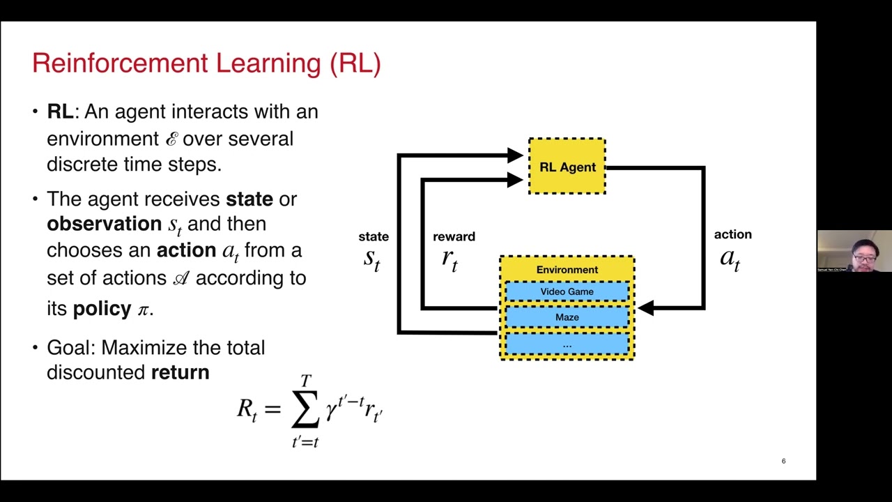
Reinforcement Learning (RL) is a subset of machine learning where an agent learns to make decisions by performing actions in an environment to maximize cumulative rewards. MATLAB, with its powerful computational abilities and specialized toolboxes, offers an extensive platform for developing, training, and deploying RL models.

1. Setting Up Your MATLAB Environment

1.1. Install MATLAB and Required Toolboxes

Before diving into RL model development, ensure that you have MATLAB installed along with the necessary toolboxes:

Reinforcement Learning Toolbox: Provides functions and tools for designing, training, and simulating RL agents.
Deep Learning Toolbox: Facilitates the creation and training of deep neural networks used in advanced RL algorithms.
Simulink (optional but recommended for complex environments): Enables the modeling and simulation of dynamic systems.

You can verify the installation by typing ver in the MATLAB Command Window and checking the list of installed toolboxes. If any required toolbox is missing, install it via the MATLAB Add-Ons menu or the MathWorks website.

1.2. Accessing Additional Resources

MATLAB offers a plethora of resources to assist you in your RL journey:

Reinforcement Learning Designer App: A graphical interface that simplifies the design and training of RL agents without extensive coding.
MATLAB Onramp Courses: Interactive, self-paced courses that provide foundational knowledge in RL.
Extensive Documentation and Examples: Access detailed guides and example projects in the MATLAB Help Center.

2. Defining the Environment

2.1. Understanding the Environment Components

The environment in RL serves as the context within which the agent operates. It defines the state space, action space, and reward structure. Establishing a well-defined environment is crucial for effective learning. The main components include:

State Space: Represents all possible states the environment can be in.
Action Space: Defines the set of actions the agent can take.
Reward Function: Provides feedback to the agent based on its actions.

2.2. Creating or Selecting an Environment

MATLAB offers both predefined and customizable environments:

Predefined Environments: MATLAB includes several built-in environments such as CartPole, Mountain Car, and Double Integrator. These are excellent for experimenting and understanding RL principles.
Custom Environments: For specific applications, you can define custom environments using MATLAB scripts or Simulink models. This allows for greater flexibility and specificity tailored to your use case.

Example: Creating a Predefined CartPole Environment


env = rlPredefinedEnv("CartPole-Discrete");

2.3. Defining Environment Dynamics

For custom environments, specify the dynamics using state transition functions. This involves:

Step Function: Defines how the environment transitions from one state to another based on the agent's action.
Reset Function: Sets the initial state of the environment at the start of each episode.

Example: Custom Environment Template


rlCreateEnvTemplate("MyCustomEnvTemplate");
% Modify the generated template to define state transitions and reward mechanisms.

3. Designing the Reinforcement Learning Agent

3.1. Selecting the RL Algorithm

MATLAB supports a variety of RL algorithms, each suited for different types of problems:

Deep Q-Network (DQN): Ideal for environments with discrete action spaces.
Proximal Policy Optimization (PPO): Suitable for environments requiring robust policy updates.
Soft Actor-Critic (SAC): Effective in continuous action spaces and complex environments.
Deep Deterministic Policy Gradient (DDPG): Best for continuous action spaces with high-dimensional inputs.

3.2. Creating the Agent

Agents can be created programmatically or via the Reinforcement Learning Designer app. Here's how to create a DQN agent programmatically:

Specify Observation and Action Spaces:


observationInfo = getObservationInfo(env);
actionInfo = getActionInfo(env);

Create the DQN Agent:


agent = rlDQNAgent(observationInfo, actionInfo);

3.3. Configuring Agent Hyperparameters

Hyperparameters significantly impact the agent's learning efficiency and performance. Key hyperparameters include:

Learning Rate: Determines how quickly the agent updates its knowledge.
Discount Factor: Balances the importance of immediate and future rewards.
Exploration Strategy: Controls the balance between exploration and exploitation, e.g., epsilon-greedy strategy.
Experience Replay Buffer Size: Stores past experiences to break correlations during training.

Example: Setting Hyperparameters for a DQN Agent


agentOpts = rlDQNAgentOptions(...
    'SampleTime', Ts, ...
    'UseDoubleDQN', true, ...
    'ExperienceBufferLength', 1e6, ...
    'MiniBatchSize', 32, ...
    'DiscountFactor', 0.99, ...
    'LearnRate', 1e-3, ...
    'Epsilon', 1.0, ...
    'EpsilonDecay', 1e-5);
agent = rlDQNAgent(observationInfo, actionInfo, agentOpts);

4. Training the RL Agent

4.1. Defining Training Options

Training options dictate how the training process is executed. Key parameters include:

Max Episodes: The maximum number of episodes to train the agent.
Max Steps Per Episode: The maximum number of steps the agent can take in each episode.
Stop Training Criteria: Conditions under which training should cease, such as reaching an average reward threshold.
Parallel Computing (optional): Utilize multiple CPU cores or GPUs to expedite training.

Example: Setting Training Options


trainingOpts = rlTrainingOptions(...
    'MaxEpisodes', 1000, ...
    'MaxStepsPerEpisode', 500, ...
    'StopTrainingCriteria', 'AverageReward', ...
    'StopTrainingValue', 480, ...
    'Verbose', true, ...
    'Plots', 'training-progress', ...
    'UseParallel', true);

4.2. Initiating the Training Process

With the environment and agent set up, proceed to train the agent:


trainStats = train(agent, env, trainingOpts);

During training, MATLAB will display progress through various plots and statistics, allowing you to monitor the agent’s learning curve and performance metrics.

4.3. Utilizing Parallel Computing

To significantly reduce training time, especially for complex models and environments, enable parallel computing:

MATLAB can leverage multi-core processors and GPUs to perform multiple simulations simultaneously.
Set the 'UseParallel' option in the training options to true, as shown in the previous example.

5. Simulating and Evaluating the Trained Agent

5.1. Running Simulations

After training, evaluate the agent's performance by simulating its interactions within the environment:


simOpts = rlSimulationOptions('MaxSteps', 500);
experience = sim(env, agent, simOpts);

This simulation provides insights into the agent’s decision-making process and its ability to achieve the desired objectives.

5.2. Analyzing Performance Metrics

Review various performance metrics to assess the agent’s effectiveness:

Average Reward: Measures the cumulative rewards over episodes.
Success Rate: Percentage of episodes where the agent achieves the goal.
Convergence: Stability and consistency of the agent’s policy over time.

5.3. Visualization Tools

MATLAB offers several visualization tools to help interpret the agent’s performance:

Training Progress Plots: Display metrics like reward trends and loss curves during training.
State-Action Heatmaps: Visualize how the agent responds to different states.
Trajectory Plots: Show the agent’s path through the environment during simulations.

6. Deploying and Extending the RL Model

6.1. Exporting the Trained Agent

Once satisfied with the trained agent, export it to the MATLAB workspace for deployment or further analysis:


trainedAgent = getBestAgent(trainStats);

6.2. Integrating with Simulink

For real-world applications and complex system integrations, incorporate the RL agent into Simulink models:

Use the rlSimulinkEnv function to create a Simulink environment.
Connect the RL agent to the Simulink model using RL blocks.
Simulate and deploy the integrated system within Simulink for comprehensive testing and validation.

6.3. Generating Optimized Code

MATLAB allows for automatic code generation, enabling deployment of the RL agent on various hardware platforms:

Use the MATLAB Coder to convert the trained model into C/C++ code.
Deploy the generated code to embedded systems, microcontrollers, or other target platforms.

6.4. Extending Functionality

Enhance your RL model by:

Importing existing policies from frameworks like TensorFlow or PyTorch.
Implementing custom reward functions to better align with specific objectives.
Utilizing multicore processors or GPUs to accelerate training and simulations.

7. Advanced Topics and Best Practices

7.1. Reward Signal Design

The reward signal critically influences the agent’s learning process. Design rewards to:

Accurately reflect the desired outcomes.
Avoid sparse or delayed rewards that can hinder learning efficiency.
Incorporate penalties for undesirable actions to guide the agent away from them.

7.2. Hyperparameter Tuning

Optimize agent performance by meticulously tuning hyperparameters:

Experiment with different learning rates to find the optimal balance between convergence speed and stability.
Adjust the discount factor to influence the agent’s focus on immediate versus future rewards.
Modify exploration strategies to ensure adequate exploration of the state-action space.

7.3. Utilizing Parallel Computing

Leverage MATLAB’s parallel computing capabilities to expedite training:

Enable parallel simulations to utilize multiple CPU cores or GPUs.
Distribute training tasks across a computing cluster for large-scale RL problems.

7.4. Debugging and Visualization

Use visualization tools to monitor and debug the RL training process:

Plot reward trends to assess learning progress.
Visualize state-action pairs to understand the agent’s decision-making patterns.
Use trajectory plots to ensure the agent navigates the environment as expected.

Conclusion

Establishing a reinforcement learning model in MATLAB involves a systematic approach that encompasses setting up the environment, designing and training the agent, and deploying the trained model for real-world applications. MATLAB’s extensive toolboxes and resources significantly simplify this process, offering robust tools for customization, optimization, and integration. By following best practices in reward design, hyperparameter tuning, and leveraging parallel computing, you can develop highly efficient and effective RL models tailored to your specific needs.

References

For further reading and detailed guides, refer to the following resources:

Reinforcement Learning Toolbox - MATLAB
Getting Started with Reinforcement Learning Toolbox - MathWorks
Reinforcement Learning Designer - MathWorks
Reinforcement Learning Onramp | MATLAB Academy
Model-Based Reinforcement Learning Using Custom Training Loop - MathWorks