Mastering Multi-Column Conditional Formatting in Excel for Dynamic Data Analysis

Excel's conditional formatting is an incredibly powerful feature that allows you to automatically apply formatting to cells based on specific criteria. This capability transforms raw data into visually intuitive insights, making it easier to identify patterns, trends, and critical information at a glance. When dealing with large datasets spread across multiple columns, the ability to highlight cells based on specific text content becomes invaluable for quick data auditing and analysis.

This comprehensive guide will walk you through the process of creating a conditional formatting rule to highlight cells across multiple columns that contain any of four specified words. We'll explore various methods, including built-in rules and formula-based approaches, to ensure you can apply this technique effectively regardless of your Excel proficiency.

Key Insights into Multi-Word, Multi-Column Conditional Formatting

Leverage 'Text That Contains' for Simple Scenarios: For highlighting cells within a single column based on a few specific words, Excel's built-in "Highlight Cells Rules > Text That Contains" is the most straightforward method.
Employ Formulas for Advanced Control: To highlight cells across multiple columns or to check for multiple words simultaneously using a single rule, formula-based conditional formatting with functions like OR, SEARCH, and ISNUMBER provides greater flexibility and power.
Absolute vs. Relative References are Crucial: Understanding when to use absolute (e.g., $A$1) and relative (e.g., A1) cell references in your conditional formatting formulas is fundamental for ensuring rules apply correctly across your selected range.

Understanding Conditional Formatting Fundamentals

Before diving into specific techniques, it's essential to grasp the core principles of conditional formatting in Excel. This feature is located on the Home tab, within the Styles group. It allows you to set rules that, when met, automatically change the appearance of cells, such as their fill color, font color, or borders. These rules can be simple, like highlighting values greater than a certain number, or complex, involving custom formulas.

When applying conditional formatting, you first select the range of cells you want the rule to apply to. Then, you define the condition and the desired formatting. For text-based conditions, Excel offers a convenient "Text That Contains" rule, but for more intricate scenarios involving multiple words or columns, custom formulas become necessary.

Navigating to Conditional Formatting

The path to applying conditional formatting is consistent across most Excel versions:

Select the range of cells where you want the formatting to apply. This could be a single column, multiple columns, or even an entire sheet.
Go to the Home tab on the Excel ribbon.
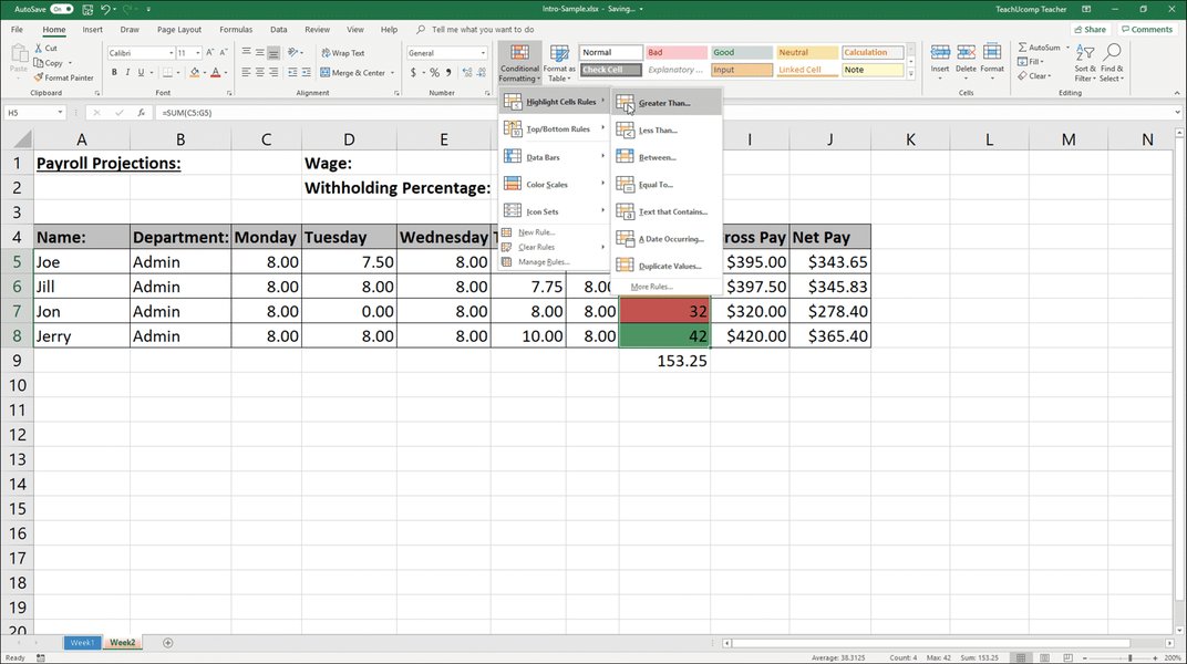
In the Styles group, click on Conditional Formatting.
From the dropdown menu, you can choose from preset rules or select New Rule for more customization.

Screenshot showing how to navigate to conditional formatting in Excel.

Navigating to the "New Rule" option within Conditional Formatting.

Highlighting Cells with Any of Four Words: Step-by-Step Methods

Method 1: Using "Text That Contains" (Best for Single Column, Few Words)

While this method is primarily designed for single words or a limited set within a single column, it's worth understanding for its simplicity. For multiple words, you'd typically create a separate rule for each word, which can become cumbersome for many words or columns.

Step-by-Step Application:

Select the Range: Highlight the column(s) where you want to apply the formatting. For instance, if your data is in columns A, B, and C, select A:C.
Access Conditional Formatting: Go to Home > Conditional Formatting > Highlight Cells Rules > Text That Contains...
Enter Words (One by One): A dialog box will appear. Enter your first word (e.g., "Apple"). Choose your desired formatting (e.g., Light Red Fill with Dark Red Text). Click OK.
Repeat for Each Word: Repeat steps 2 and 3 for each of the remaining three words you want to highlight. Each word will require a separate rule.

Limitation: This method creates multiple rules, which can be less efficient and harder to manage if you have many words or need to apply the same logic across numerous columns.

Method 2: Using a Formula with OR and SEARCH (Recommended for Multiple Words and Columns)

This is the most flexible and efficient method for highlighting cells across multiple columns that contain any of four specific words. It uses a formula-based rule, which allows you to define complex conditions.

Understanding the Formula:

The core of this method lies in combining the OR function with multiple SEARCH functions. The SEARCH function looks for a text string within another text string and returns the starting position of the first text string. If the text is not found, it returns a #VALUE! error. The ISNUMBER function checks if the result of SEARCH is a number (meaning the word was found). Finally, OR checks if any of these conditions are true.

The general formula structure would look like this:

\[ \text{=OR(ISNUMBER(SEARCH("word1", A1)), ISNUMBER(SEARCH("word2", A1)), ISNUMBER(SEARCH("word3", A1)), ISNUMBER(SEARCH("word4", A1)))} \]

Where "word1", "word2", "word3", and "word4" are your specific keywords, and A1 is the top-left cell of your selected range (the "active cell" when you create the rule). By using a relative reference like A1, Excel automatically adjusts the formula for each cell in your selected range (e.g., A2, B1, B2, etc.).

Step-by-Step Application:

Select the Entire Target Range: Carefully select all the cells across multiple columns where you want the conditional formatting to apply. For example, if your data spans columns A through D and rows 2 through 100, select A2:D100. Ensure that the very first cell you selected (e.g., A2) is the active cell (it will typically appear lighter than the rest of the selected range).
Open New Rule Dialog: Go to Home > Conditional Formatting > New Rule...
Choose "Use a formula to determine which cells to format": In the "New Formatting Rule" dialog box, select this option.
Enter the Formula: In the "Format values where this formula is true:" box, type your formula. For example, if your four words are "Apple", "Banana", "Cherry", and "Date", and your selected range starts at cell A1, the formula would be:
```
=OR(ISNUMBER(SEARCH("Apple",A1)),ISNUMBER(SEARCH("Banana",A1)),ISNUMBER(ISNUMBER(SEARCH("Cherry",A1))),ISNUMBER(SEARCH("Date",A1)))
```
Important Note on Case-Sensitivity: The SEARCH function is not case-sensitive. If you need a case-sensitive search, use the FIND function instead of SEARCH.
Set the Formatting: Click the Format... button. Choose your desired fill color, font style, border, etc., then click OK.
Apply the Rule: Click OK in the "New Formatting Rule" dialog box. The formatting will be applied to all cells in your selected range that contain any of the specified words.

Method 3: Using a Named Range for Keywords (Advanced and Scalable)

For scenarios where your list of keywords might change frequently, or if you have more than a few words, creating a named range for your keywords can significantly streamline the process and make your conditional formatting rules more dynamic.

Step-by-Step Application:

Create Your Keyword List: In a separate column (or even a separate sheet), list your four words. For example, in cell G1, type "Apple"; in G2, "Banana"; in G3, "Cherry"; and in G4, "Date".
Create a Named Range: Select the cells containing your keywords (e.g., G1:G4). In the Name Box (to the left of the formula bar), type a name for this range, such as MyKeywords, and press Enter.
Select Target Range and New Rule: Select the cells in your main data sheet where you want to apply the formatting (e.g., A2:D100). Go to Home > Conditional Formatting > New Rule... > Use a formula to determine which cells to format.
Enter the Formula: Use the SUMPRODUCT function in combination with ISNUMBER and SEARCH, referencing your named range. The formula becomes much cleaner:
```
=SUMPRODUCT(--ISNUMBER(SEARCH(MyKeywords,A1)))>0
```
Here, MyKeywords refers to your named range. The -- (double unary) converts TRUE/FALSE values to 1/0, and SUMPRODUCT sums them up. If the sum is greater than 0, it means at least one keyword was found.
Set Formatting and Apply: Click Format... to choose your desired style, then click OK twice to apply the rule.

This method is highly scalable. If you need to add or remove keywords, you just update the named range, and the conditional formatting rule automatically adapts without needing to be edited.

Managing and Prioritizing Conditional Formatting Rules

When you have multiple conditional formatting rules applied to the same range, their order of precedence matters. Excel processes rules from top to bottom in the Conditional Formatting Rules Manager. If a cell meets the criteria for more than one rule, the rule higher up in the list (with a higher priority) will be applied. You can change the order of rules using the up and down arrows in the Rules Manager.

Additionally, the Stop If True option can be very useful. If this option is checked for a rule, Excel will stop processing further rules for that cell once the current rule's condition is met. This can be beneficial for performance in large datasets and for ensuring specific formatting overrides others.

Screenshot of the Conditional Formatting Rules Manager showing options to manage rules.

The Conditional Formatting Rules Manager allows you to organize and prioritize your rules.

Applying Rules to Entire Rows Based on Cell Content

Sometimes, you might want to highlight an entire row if a cell within that row contains one of your four words. The key to this is using absolute references correctly in your formula.

Formula Adjustment for Entire Rows:

If you select an entire range of rows (e.g., A2:Z100) and want the formatting to apply to the whole row if a specific column (e.g., column C) contains one of your words, the formula needs to lock the column reference, but allow the row reference to change:

\[ \text{=OR(ISNUMBER(SEARCH("word1", \$C2)), ISNUMBER(SEARCH("word2", \$C2)), ISNUMBER(SEARCH("word3", \$C2)), ISNUMBER(SEARCH("word4", \$C2)))} \]

Notice the $C2. The $ before C makes the column reference absolute, so Excel always looks in column C for the word. The absence of a $ before 2 keeps the row reference relative, allowing it to adjust as the rule is applied down each row (C3, C4, etc.).

Advanced Considerations and Tips

When working with conditional formatting on a large scale, especially across many columns and rows, performance can become a factor. Complex formulas or a high number of rules can slow down your spreadsheet. Here are some advanced tips:

Optimize Formulas: Ensure your formulas are as efficient as possible. Avoid volatile functions if not strictly necessary.
Test on Small Ranges: Before applying conditional formatting to your entire dataset, test your rule on a smaller subset to ensure it behaves as expected.
Use Helper Columns: For extremely complex conditions, consider using a helper column to perform calculations, and then base your conditional formatting rule on the result in the helper column. You can hide the helper column if it's not needed for display.
VBA for Very Specific Needs: For highly customized highlighting, such as highlighting only a portion of text within a cell (not the entire cell), VBA (Visual Basic for Applications) might be necessary. However, this requires basic coding skills.

Performance Evaluation of Conditional Formatting Methods

To give you a better sense of which method might be suitable for different scenarios, consider the following radar chart. It rates each method based on criteria like ease of use, scalability, flexibility, and potential performance impact.

The radar chart illustrates the strengths and weaknesses of each approach. "Text That Contains" is easy for simple cases but struggles with scalability. The formula with OR and SEARCH offers a good balance of flexibility and scalability. The named range method, while requiring a slightly steeper initial learning curve, provides the best scalability and dynamic capabilities for managing a large or frequently changing list of keywords.

Summary of Conditional Formatting Rules and Their Use Cases

To help you choose the best approach, here's a table summarizing the different methods and their ideal use cases:

Method	Description	Ideal Use Case	Pros	Cons
Highlight Cells Rules > Text That Contains	Built-in rule for single word or simple text strings. Requires multiple rules for multiple words.	Highlighting cells in a single column for 1-3 specific, unchanging words.	Very easy to set up, no formula knowledge required.	Not scalable for many words or columns, creates many individual rules.
Formula with OR and SEARCH	Uses a custom formula combining `OR(ISNUMBER(SEARCH()))` for multiple text strings.	Highlighting cells across multiple columns for 4+ words, where keywords are relatively stable.	More flexible, single rule for multiple words, applies easily across columns.	Requires understanding of basic Excel formulas.
Formula with Named Range (SUMPRODUCT, ISNUMBER, SEARCH)	Uses a custom formula that references a dynamic list of keywords in a named range.	Highlighting cells for a large, frequently changing list of keywords across multiple columns.	Highly scalable, keywords are easy to update, single powerful rule.	Slightly more complex setup with named ranges, formula can appear daunting to beginners.

Visualizing Conditional Formatting Techniques

This video provides a practical demonstration of using conditional formatting with multiple conditions, which directly applies to highlighting cells based on multiple words across columns. It offers a visual walkthrough that can reinforce the concepts discussed in the formula-based methods.

A visual guide on using conditional formatting with multiple conditions in Excel.

Frequently Asked Questions

How do I highlight only part of the text within a cell, not the whole cell?

Excel's conditional formatting highlights the entire cell. To highlight only specific words within a cell, you would typically need to use VBA (Visual Basic for Applications) scripting. This allows for more granular text formatting but requires basic programming knowledge.

Can I use wildcards with conditional formatting text rules?

When using the "Text That Contains" rule, it inherently functions as a wildcard search (e.g., searching for "app" will highlight "Apple", "application", etc.). When using formulas with SEARCH, the * wildcard isn't typically used directly within the SEARCH function itself for this purpose, as SEARCH already finds substrings.

My conditional formatting isn't working. What should I check?

Common issues include: incorrect cell range selection (especially the active cell when creating a formula-based rule), errors in the formula (check for typos, proper use of $ for absolute/relative references), or conflicting rules in the Conditional Formatting Rules Manager. Always ensure the formula evaluates to TRUE/FALSE.

How can I apply the same conditional formatting rule to many different, non-contiguous columns?

You can select all non-contiguous columns by holding down the Ctrl key while clicking on each column header. Then, apply the conditional formatting rule as you normally would. Excel will apply the rule to all selected columns. Alternatively, apply the rule to one column, then use the Format Painter to copy the formatting to other columns.

Conclusion

Conditional formatting is an indispensable tool in Excel for making your data more digestible and actionable. By mastering the techniques for highlighting cells based on multiple text values across multiple columns, you can significantly enhance your ability to analyze and present information. Whether you choose the simpler "Text That Contains" for straightforward needs or delve into formula-based solutions with OR, SEARCH, or named ranges for more complex scenarios, the flexibility of Excel ensures you can always bring your most important data points to the forefront.