Ithy - Unlock Excel's Data-Finding Powerhouse: What is VLOOKUP?

The VLOOKUP function in Microsoft Excel is a fundamental tool for anyone working with data tables. Standing for "Vertical Lookup," it allows you to search for a specific piece of information in one column and retrieve a corresponding value from a different column in the same row. Think of it as Excel's way of automatically finding related data, saving you countless hours of manual searching, especially in large datasets.

Key Takeaways

Vertical Search: VLOOKUP searches vertically down the first column of a specified data range (table array).
Data Retrieval: When it finds a match for your lookup value, it moves across that row to retrieve data from a column you designate.
Exact vs. Approximate Match: You can specify whether VLOOKUP should find an exact match (most common use) or an approximate match (useful for ranges).

Decoding the VLOOKUP Syntax

To use VLOOKUP effectively, you need to understand its structure, known as syntax. The function requires specific pieces of information, called arguments, provided in a precise order:

=VLOOKUP(lookup_value, table_array, col_index_num, [range_lookup])

Understanding the Arguments

Each part of the VLOOKUP formula plays a crucial role. Here's a breakdown:

Argument	Description	Example
`lookup_value`	The specific value you want to search for. This value must exist in the first column of your `table_array`. It can be a cell reference (e.g., `A2`), a number (e.g., `101`), or text (e.g., `"Apple"` - text must be in quotes).	`A2` or `"Product ID 123"`
`table_array`	The range of cells containing the data you want to search within. This range must include both the column with the `lookup_value` (which must be the leftmost column in this range) and the column containing the value you want to retrieve.	`A1:D100` or `Sheet2!B2:F50`
`col_index_num`	The column number within the `table_array` from which you want to retrieve the corresponding value. The first column of the `table_array` is column 1, the second is 2, and so on.	`3` (to get data from the third column of the `table_array`)
`[range_lookup]`	An optional argument determining the match type. Enter `FALSE` for an exact match (looks for the exact `lookup_value`). Enter `TRUE` or omit the argument for an approximate match (finds the largest value less than or equal to the `lookup_value`; requires the first column of `table_array` to be sorted numerically or alphabetically). Most common use cases require `FALSE`.	`FALSE` (for exact match) or `TRUE` (for approximate match)

Important Note on Case Sensitivity

VLOOKUP is not case-sensitive. It treats "apple", "Apple", and "APPLE" as the same when searching for the lookup_value.

How VLOOKUP Works: The Search Process

Understanding the step-by-step process helps in troubleshooting and applying the function correctly:

Identify the Target: Excel takes your lookup_value.
Scan Vertically: It scans down the first column of the specified table_array, looking for a match to the lookup_value.
Locate the Row: Once it finds the first matching value, it stops scanning that column.
Move Horizontally: It then moves across that same row to the column number specified by col_index_num.
Return the Value: Excel returns the value found in the cell at the intersection of the matched row and the specified column number.
Handle No Match: If no match is found (especially when using FALSE for exact match), VLOOKUP returns the #N/A error.

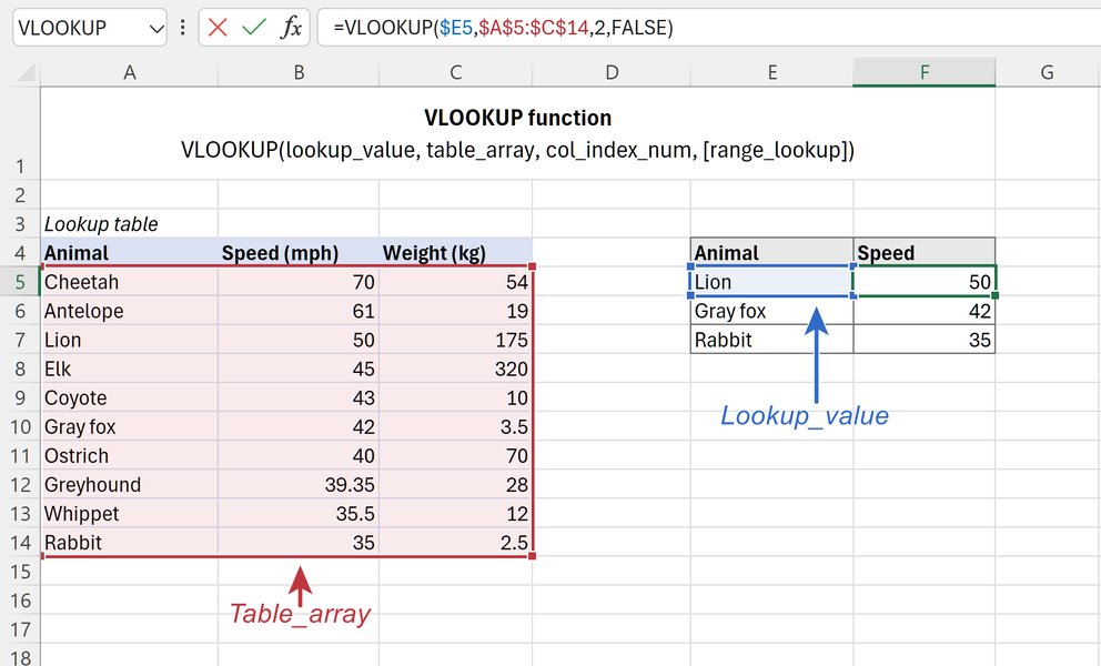
Diagram illustrating the VLOOKUP function arguments in Excel

Visual breakdown of the VLOOKUP function's arguments.

Exact vs. Approximate Matches: Choosing Your Search Type

The range_lookup argument significantly changes how VLOOKUP behaves.

Exact Match (FALSE)

This is the most common setting. Use FALSE when you need to find a unique identifier like an employee ID, product code, or specific name. VLOOKUP will search for the exact lookup_value in the first column. If it doesn't find an identical match, it returns #N/A. The order of data in the first column doesn't matter for an exact match.

Example: =VLOOKUP(105, A1:C10, 2, FALSE) looks for the exact value 105 in column A and returns the corresponding value from column B.

Approximate Match (TRUE or Omitted)

Use TRUE (or omit the argument) when looking for a value within a range, like finding a tax rate based on income level or a grade based on a score. For this to work correctly, the first column of your table_array must be sorted in ascending order (numerically or alphabetically).

VLOOKUP finds the largest value in the first column that is less than or equal to your lookup_value. If your lookup_value is smaller than the smallest value in the first column, it returns #N/A.

Example: =VLOOKUP(75, A1:B5, 2, TRUE) where column A contains scores (0, 60, 70, 80, 90) and column B contains grades (F, D, C, B, A). It would look for 75, find the largest value less than or equal to it (70), and return the corresponding grade "C".

Visualizing VLOOKUP Concepts

This mindmap provides a quick overview of the key elements associated with the VLOOKUP function.

mindmap root["Excel VLOOKUP Function"] Purpose["Search & Retrieve Data"] id1["Find value in first column"] id2["Return value from same row, different column"] id3["Automate data lookup"] Syntax["=VLOOKUP(lookup_value, table_array, col_index_num, [range_lookup])"] arg1["lookup_value: What to find"] arg2["table_array: Where to look (lookup in 1st col)"] arg3["col_index_num: Which column's data to return (1=first)"] arg4["range_lookup: Match type (Optional)"] Match_Types["Exact vs. Approximate"] exact["FALSE: Exact match required
(Most common)"] approx["TRUE/Omitted: Approximate match
(Requires sorted 1st column)"] Key_Limitations["Constraints"] lim1["Only looks right (cannot retrieve from left columns)"] lim2["Looks in first column ONLY of table_array"] lim3["Returns only the FIRST match found (if duplicates exist)"] lim4["Can be slow on very large datasets"] Alternatives["More Flexible Functions"] alt1["INDEX / MATCH (More versatile, looks left/right)"] alt2["XLOOKUP (Newer, simpler, more powerful)"]

Practical Examples and Use Cases

Common Scenarios

Fetching Employee Details: Look up an employee's name, department, or salary using their unique ID. Formula: =VLOOKUP(EmployeeID_Cell, EmployeeTableRange, NameColumnNumber, FALSE).
Product Information Lookup: Find the price or stock level of a product based on its SKU or product name. Formula: =VLOOKUP("ProductSKU", ProductListRange, PriceColumnNumber, FALSE).
Combining Data from Different Sheets: Pull sales figures from one sheet into a summary report on another sheet based on a common identifier like a region or date. Formula: =VLOOKUP(A2, Sheet2!A1:D50, 4, FALSE).
Grading or Tiered Pricing: Assign grades based on scores or determine commission rates based on sales tiers using an approximate match. Formula: =VLOOKUP(ScoreCell, GradeTableRange, GradeColumnNumber, TRUE).

Using Wildcards for Partial Matches

VLOOKUP supports wildcards (* for any sequence of characters, ? for any single character) when using an exact match (FALSE) if the lookup_value is text.

"Apple*" matches "Apple", "Apples", "Apple Pie".
"Sm?th" matches "Smith", "Smyth".

Example: =VLOOKUP("Corp*", A1:B10, 2, FALSE) finds the first entry starting with "Corp" in column A.

Tips for Effective VLOOKUP Use

Absolute References: When copying a VLOOKUP formula down a column, use absolute references (e.g., $A$1:$D$100) for the table_array to prevent the range from shifting. Press F4 after selecting the range to toggle absolute references.
Sort for Approximate Match: Remember to sort the first column of your table_array in ascending order if using TRUE for approximate matching.
Error Handling: Wrap your VLOOKUP in the IFERROR function to display a custom message instead of #N/A when a value isn't found. Example: =IFERROR(VLOOKUP(A2, B1:D10, 2, FALSE), "Not Found").
Check Data Types: Ensure the lookup_value and the data in the first column of the table_array have matching data types (e.g., both are numbers or both are text). Numbers stored as text can cause errors.
Trim Spaces: Extra spaces before or after values can prevent matches. Use the TRIM function to clean data if necessary.

Understanding VLOOKUP's Limitations

While incredibly useful, VLOOKUP has limitations that are important to be aware of:

Looks Right Only: VLOOKUP can only retrieve data from columns to the right of the lookup column within the table_array. It cannot look to the left.
First Column Dependency: The column containing the value you want to search for (lookup_value) must be the first (leftmost) column in the defined table_array.
First Match Only: If there are duplicate values in the first column, VLOOKUP will only find and return the result corresponding to the first match it encounters when scanning from top to bottom.
Performance: On very large datasets (hundreds of thousands of rows), VLOOKUP can sometimes be slower than alternative methods like INDEX/MATCH.
Column Insertion/Deletion Issues: If columns are inserted or deleted within the table_array, the hardcoded col_index_num might become incorrect, leading to wrong results.

Exploring Alternatives: INDEX/MATCH and XLOOKUP

Due to VLOOKUP's limitations, Excel offers more flexible alternatives:

INDEX and MATCH

This combination of two functions is often considered superior to VLOOKUP because:

It can look up values in any column and return values from any other column (left or right).
It's more resilient to changes in spreadsheet structure (inserting/deleting columns).
It can perform horizontal lookups (using MATCH within HLOOKUP or INDEX) and two-way lookups.

The typical structure is: =INDEX(ReturnColumnRange, MATCH(LookupValue, LookupColumnRange, 0)) (The 0 in MATCH specifies an exact match).

XLOOKUP

Introduced in newer versions of Excel (Microsoft 365, Excel 2021), XLOOKUP is designed to replace VLOOKUP, HLOOKUP, and INDEX/MATCH for many scenarios. Its advantages include:

Simpler syntax.
Defaults to an exact match (no need to specify FALSE).
Can look up and return values in any direction (left, right, up, down).
Can return entire rows or columns, not just single values.
Includes built-in error handling options.

Basic syntax: =XLOOKUP(lookup_value, lookup_array, return_array, [if_not_found], [match_mode], [search_mode])

Lookup Function Comparison

This chart provides a relative comparison of VLOOKUP, INDEX/MATCH, and XLOOKUP across several key attributes based on typical usage scenarios. Higher scores indicate better performance or greater flexibility in that area.

While VLOOKUP remains highly relevant and widely used, especially in environments with older Excel versions, understanding its limitations and the capabilities of INDEX/MATCH and XLOOKUP allows you to choose the best tool for your specific data lookup task.

Watch a VLOOKUP Tutorial

For a visual guide and practical demonstration, check out this official tutorial from Microsoft Excel on how to use the VLOOKUP function:

This video provides examples and walks through the process of setting up and using VLOOKUP for common data retrieval tasks, reinforcing the concepts explained above.

References

Last updated May 5, 2025