Flow Matching Generative Models: A Comprehensive Overview

Flow matching generative models represent a cutting-edge approach in the field of machine learning, offering a powerful and flexible framework for generating complex data distributions. These models synthesize elements from continuous normalizing flows (CNFs) and diffusion models, providing a streamlined yet robust method for transforming simple probability distributions into intricate, high-dimensional data distributions. This comprehensive overview will delve into the theoretical underpinnings, architectural design, training methodologies, diverse applications, advantages, and limitations of flow matching generative models.

Theoretical Foundations

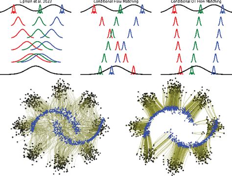
Flow matching is fundamentally rooted in the principles of optimal transport and differential flows. It aims to model a probability density path that smoothly transforms a simple prior distribution, such as a Gaussian, into a complex target data distribution. This transformation is achieved through a time-dependent diffeomorphic map, referred to as a "flow."

Key Concepts

1. Probability Density Transformation: Flow matching operates by defining a continuous path in the space of probability distributions. This path starts at a simple base distribution, ( p_0(x) ) (e.g., a standard normal distribution), and evolves over time to reach the target distribution, ( p_T(x) ), which represents the complex data distribution to be modeled.
2. Vector Fields and Flows: Instead of directly modeling the flow, flow matching focuses on its time derivative, which is represented as a vector field, ( v_t(x) ). This vector field dictates the velocity of the flow at any given point ( x ) and time ( t ). Mathematically, the evolution of the flow is governed by the ordinary differential equation (ODE):
   [ \frac{\partial x_t}{\partial t} = v_t(x_t), ]
   where ( x_t ) represents the data at time ( t ).
3. Optimal Transport and Matching: The core objective of flow matching is to minimize the discrepancy between the learned flow, ( v_t(x) ), and the ideal flow that would perfectly transport ( p_0(x) ) to ( p_T(x) ). This discrepancy is quantified using an objective function derived from the continuity equation:
   [ \frac{\partial p_t(x)}{\partial t} + \nabla \cdot (p_t(x) v_t(x)) = 0, ]
   where ( p_t(x) ) is the intermediate distribution at time ( t ). This equation ensures that the learned flow conserves mass and accurately matches the target distribution.
4. Conditional Velocities: Flow matching simplifies the learning process by regressing onto conditional velocities. These velocities are derived from simple conditional vector fields that interpolate between the reference and target distributions, making them easier to evaluate and integrate over time.
5. Marginalization: The target vector field is constructed as the marginalization of these conditional vector fields. This ensures that the learned flow remains consistent with the target distribution throughout the transformation process.

Mathematical Formulation

The flow matching objective is typically expressed as a minimization problem:
[ \min_{\theta} \mathbb{E}_{x \sim q(x)} \left[ \| v_\theta(x, t) - v^*(x, t) \|^2 \right] ]
where ( v_\theta(x, t) ) is the neural network parameterizing the vector field, and ( v^*(x, t) ) represents the ground-truth conditional velocity. This objective aims to minimize the mean squared error (MSE) between the predicted velocities and the ground-truth velocities.

The theoretical framework of flow matching draws heavily from the change of variables formula, which is fundamental to normalizing flows. This formula allows for the exact computation of the log-likelihood of the data, a significant advantage over other generative models like GANs, which do not provide direct likelihood estimates. The change of variables formula is given by:
[ p_X(x) = p_Z(f^{-1}(x)) \left| \det \left( \frac{\partial f^{-1}(x)}{\partial x} \right) \right| ]
where ( p_X(x) ) is the target distribution, ( p_Z(z) ) is the base distribution, ( f ) is the transformation function, and ( \det ) denotes the determinant of the Jacobian matrix of ( f^{-1} ).

Architecture

The architecture of flow matching models is centered around a neural network that parameterizes the vector field governing the flow. This architecture typically comprises the following components:

Neural Network Parameterization

The core of the flow matching model is a neural network, denoted as ( v_\theta(x, t) ), where ( \theta ) represents the learnable parameters. This network takes as input the data point ( x ) and the time variable ( t ) and outputs the velocity vector at that specific point in space and time. The choice of neural network architecture can vary, but it often involves deep, fully connected layers or convolutional layers for image data.

Time Conditioning

To ensure that the flow field evolves smoothly and coherently over time, flow matching models incorporate time conditioning mechanisms. These mechanisms can include:

• Positional Encodings: Similar to those used in transformer models, positional encodings provide the network with information about the current time step.
• Learnable Embeddings: Each time step can be associated with a learnable embedding vector that is fed into the network.
• Sinusoidal Functions: Sinusoidal functions of time can be used to encode temporal information, providing a continuous and differentiable representation of time.

Condition Encoder

For conditional generative tasks, where the generation process is guided by auxiliary information (e.g., class labels, numerical properties), a condition encoder is integrated into the architecture. This encoder maps the auxiliary information into a latent space, which is then used to modulate the vector field. This allows the model to generate data that is consistent with the provided conditions.

ODE Solver

During inference, the learned vector field is used in conjunction with an ordinary differential equation (ODE) solver to generate new samples. The ODE solver numerically integrates the vector field over time, starting from a sample drawn from the base distribution and following the flow until it reaches the target distribution. Popular ODE solvers include Runge-Kutta methods and Euler integration.

Regularization Layers

To stabilize the training process and improve the generalization capabilities of the model, flow matching models often incorporate regularization techniques. These can include:

• Weight Normalization: Normalizing the weights of the neural network can help prevent exploding or vanishing gradients.
• Spectral Normalization: This technique controls the Lipschitz constant of the network, ensuring smoother transformations.
• Gradient Clipping: Limiting the magnitude of gradients during training can prevent instability.

Extensions to Non-Euclidean Domains

Recent advancements have extended flow matching to non-Euclidean geometries, such as manifolds and graphs. This enables applications in domains like molecular generation and physics simulations, where the data naturally resides in non-Euclidean spaces. These extensions often involve adapting the vector field and ODE solver to operate on manifolds or graphs, requiring specialized architectures and mathematical formulations.

Training Processes

The training process for flow matching models is designed to be efficient and scalable. It involves optimizing the neural network ( v_\theta(x, t) ) to minimize a loss function that measures the discrepancy between the learned flow and the ideal flow. The key steps in the training process are as follows:

Data Preparation

The training process begins by sampling data points from the target distribution, ( q(x) ), and the reference distribution, ( p(x) ). These samples are used to compute the conditional velocities that define the desired flow from the reference to the target distribution.

Conditional Velocity Estimation

The ground-truth conditional velocities, ( v^*(x, t) ), are computed using analytical or empirical methods. These velocities represent the ideal flow that the model aims to learn. For simple cases, analytical solutions may be available. In more complex scenarios, empirical methods, such as kernel density estimation, can be used to approximate the conditional velocities.

Loss Function

The primary loss function used in flow matching is derived from the continuity equation and measures the mean squared error (MSE) between the predicted velocities, ( v_\theta(x, t) ), and the ground-truth velocities, ( v^*(x, t) ). The loss function can be expressed as:
[ \mathcal{L}(\theta) = \mathbb{E}_{x, t} \left[ \| v_\theta(x, t) - v^*(x, t) \|^2 \right] ]
This loss function encourages the model to learn a vector field that closely matches the ideal flow.

Optimization

Gradient-based optimization techniques, such as Adam or RMSProp, are used to update the parameters ( \theta ) of the neural network. The training process is iterative and involves computing the gradients of the loss function with respect to the parameters and updating the parameters accordingly. Careful tuning of hyperparameters, such as learning rate, batch size, and regularization strength, is crucial for successful training.

Regularization

Regularization techniques, such as weight decay and gradient clipping, are employed during training to ensure stability and prevent overfitting. These techniques help the model generalize better to unseen data and improve the overall quality of the generated samples.

Post-Training Fine-Tuning

After the initial training phase, the model can be further fine-tuned using techniques like adversarial training or importance sampling. Adversarial training involves introducing an adversarial loss that encourages the model to generate samples that are indistinguishable from real data. Importance sampling can be used to refine the model's estimates of the target distribution, improving the accuracy of the generated samples.

Evaluation Metrics

The performance of flow matching models is typically evaluated using metrics such as:

• Log-Likelihood: The log-likelihood of the generated samples under the target distribution provides a measure of how well the model has learned the underlying data distribution.
• Fréchet Inception Distance (FID): For image generation tasks, FID is a widely used metric that compares the statistics of generated images to those of real images.
• Perceptual Quality Metrics: For audio and video synthesis, perceptual quality metrics, such as the Perceptual Evaluation of Speech Quality (PESQ), can be used to assess the quality of the generated samples.

Applications

Flow matching models have demonstrated remarkable versatility and effectiveness across a wide range of applications:

Image Generation

Flow matching models excel at generating high-quality images by learning the underlying distribution of natural images. They have been successfully applied to tasks such as:

• Super-Resolution: Enhancing the resolution of low-resolution images.
• Inpainting: Filling in missing or corrupted regions of images.
• Style Transfer: Applying the style of one image to the content of another.
• Image-to-Image Translation: Converting images from one domain to another (e.g., sketches to photos).

Video Synthesis

By extending the flow field to the temporal domain, flow matching models can synthesize realistic video sequences. They capture both the spatial and temporal dynamics of video data, enabling the generation of coherent and visually appealing videos. Applications include:

• Video Prediction: Predicting future frames in a video sequence.
• Video Interpolation: Generating intermediate frames to create smooth transitions.
• Video Editing: Modifying the content or style of existing videos.

Audio and Speech Generation

Flow matching models have been used to generate high-fidelity audio signals, including speech synthesis and music generation. They excel in capturing the fine-grained temporal structure of audio data, resulting in natural-sounding and expressive audio. Applications include:

• Text-to-Speech (TTS): Converting text into natural-sounding speech.
• Voice Conversion: Transforming the voice of one speaker to sound like another.
• Music Generation: Creating novel musical pieces in various styles.

Biological Data Modeling

In bioinformatics, flow matching models have been applied to tasks such as protein structure prediction and molecular generation. The complex, multi-modal nature of biological data makes it well-suited for flow matching, which can effectively model these intricate distributions. Applications include:

• Protein Folding: Predicting the 3D structure of proteins from their amino acid sequences.
• Drug Discovery: Generating novel molecules with desired properties for pharmaceutical applications.
• Genomic Data Analysis: Modeling the distribution of genomic sequences and identifying patterns.

Text Generation

Although less common, flow matching models have also been explored for natural language processing tasks. They offer an alternative to autoregressive and diffusion-based approaches for text generation and machine translation. Applications include:

• Text Generation: Creating coherent and contextually relevant text.
• Machine Translation: Translating text from one language to another.
• Dialogue Generation: Generating responses in a conversational setting.

Advantages

Flow matching offers several significant advantages over traditional generative modeling frameworks:

Continuous and Deterministic

Unlike stochastic models like GANs or diffusion models, flow matching provides a continuous and deterministic mapping from the base distribution to the target distribution. This deterministic nature leads to more stable and interpretable results. The continuous flow allows for smooth interpolation between samples and provides a clear path from noise to data.

Scalability

Flow matching models are highly scalable and can handle high-dimensional data efficiently. This makes them suitable for applications like video synthesis and 3D modeling, where the data dimensionality is inherently large. The ability to leverage GPU acceleration and parallelization further enhances their scalability.

Theoretical Rigor

The framework of flow matching is grounded in well-established mathematical principles, including optimal transport and differential flows. This provides a solid theoretical foundation for its design and analysis, making it easier to understand and reason about the model's behavior.

Flexibility

Flow matching models can be easily adapted to different data modalities and tasks by modifying the architecture and loss function. This flexibility allows them to be applied to a wide range of domains, from images and videos to audio and biological data. The ability to incorporate conditional information further enhances their adaptability.

Simplicity

Compared to diffusion models, flow matching offers a simpler and more straightforward approach to generative modeling. It avoids the need for complex noise schedules and score estimation, resulting in a more streamlined training process and easier implementation.

Efficiency

Flow matching models are computationally efficient, requiring fewer training iterations and less memory compared to diffusion models. The simpler trajectories used in flow matching reduce computational complexity, and the more direct path between the prior and target distributions leads to faster convergence during training.

Interpretability

The learned vector field in flow matching provides a clear geometric interpretation of the transformation from the reference distribution to the target distribution. This interpretability can be valuable for understanding the underlying structure of the data and for debugging the model.

Limitations

Despite their numerous strengths, flow matching models have certain limitations:

Computational Complexity

Training flow matching models can be computationally expensive, especially for high-dimensional data. The need to compute gradients and solve differential equations adds to the computational burden. While they are generally more efficient than diffusion models, the computational cost can still be significant for complex applications.

Sensitivity to Hyperparameters

The performance of flow matching models is highly sensitive to hyperparameter choices, such as learning rate, batch size, and regularization strength. This can make training challenging and time-consuming, requiring careful tuning and experimentation to achieve optimal results.

Limited Adoption

As a relatively new framework, flow matching has not yet achieved widespread adoption in the research community. This limits the availability of pre-trained models and open-source implementations compared to more established methods like GANs and VAEs. However, the growing interest in flow matching suggests that this limitation may be temporary.

Lack of Robustness

Flow matching models may struggle with out-of-distribution data or adversarial inputs. They rely on the assumption that the target distribution is well-represented in the training data. When this assumption is violated, the model's performance can degrade significantly. Developing more robust flow matching models is an active area of research.

ODE Solver Overhead

The reliance on ODE solvers can introduce computational overhead during inference, especially for high-dimensional data. While ODE solvers are generally efficient, they can still add to the overall computational cost of generating samples. Research into more efficient ODE solvers or alternative integration methods could help mitigate this limitation.

Training Stability

Training flow matching models can be sensitive to hyperparameters, requiring careful tuning to ensure stability. Instabilities during training can lead to poor convergence or suboptimal results. Techniques such as gradient clipping and careful initialization can help improve training stability, but further research is needed to develop more robust training methodologies.

Non-Euclidean Challenges

Extending flow matching to non-Euclidean domains, such as manifolds and graphs, requires additional theoretical and computational considerations. Adapting the vector field and ODE solver to operate in these spaces can be complex and may require specialized architectures and mathematical formulations. While progress has been made in this area, further research is needed to fully realize the potential of flow matching in non-Euclidean settings.

Conclusion

Flow matching represents a significant advancement in the field of generative modeling, offering a powerful and flexible framework for synthesizing complex data. Its theoretical foundations in optimal transport and differential flows provide a rigorous basis for its design, while its neural network-based architecture enables scalability and adaptability. Flow matching has demonstrated impressive performance across a wide range of applications, from image and video generation to audio synthesis and biological data modeling. Its advantages, including continuity, scalability, theoretical rigor, flexibility, simplicity, efficiency, and interpretability, make it a compelling alternative to traditional generative models.

Despite its limitations, such as computational complexity, sensitivity to hyperparameters, limited adoption, lack of robustness, ODE solver overhead, training stability challenges, and complexities in non-Euclidean domains, flow matching holds great promise for the future of generative modeling. Ongoing research aimed at addressing these limitations and further exploring the capabilities of flow matching is likely to yield even more powerful and versatile generative models in the years to come. As the field continues to evolve, flow matching is poised to play an increasingly important role in a variety of applications, driving innovation and advancing the state of the art in machine learning and artificial intelligence.

For further details and resources, refer to the following:

• Meta AI's Flow Matching Guide and Code: Flow Matching Guide and Code
• Cambridge MLG Blog on Flow Matching: Flow Matching
• NeurIPS 2024 Tutorial on Flow Matching: Flow Matching Tutorial
• Scott H. Hawley's Blog on Flow Models: Flow Models
• "Variational Inference with Normalizing Flows" by Rezende and Mohamed: Variational Inference with Normalizing Flows
• "Glow: Generative Flow with Invertible 1x1 Convolutions" by Kingma and Dhariwal: Glow: Generative Flow with Invertible 1x1 Convolutions
• Distill article on GAN Open Problems: GAN Open Problems