Comprehensive Guide to Probability and Statistics for GATE Exam

Mastering Core Concepts to Ace Your GATE Probability and Statistics Section

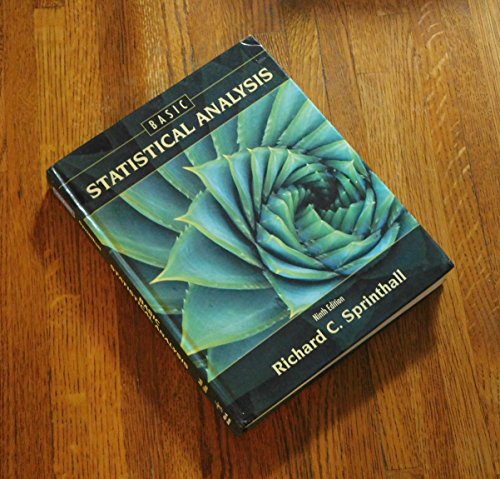
Key Takeaways

Fundamental Concepts: Understanding counting techniques, probability axioms, and various types of probabilities is essential for solving complex problems.
Statistical Measures and Distributions: Grasping measures of central tendency, dispersion, and different probability distributions aids in data analysis and interpretation.
Inferential Statistics: Mastery of the Central Limit Theorem, confidence intervals, and hypothesis testing methods like z-test, t-test, and chi-squared tests is crucial for making informed decisions based on data.

1. Counting Techniques

Permutations and Combinations

Counting techniques are foundational in probability, enabling the determination of the number of possible outcomes in various scenarios.

Permutations

Permutations refer to the arrangement of objects where the order matters. The number of ways to arrange n distinct objects is given by n! (n factorial).

Formula: P(n, r) = n! / (n – r)!

Example: The number of ways to arrange 3 objects out of 5 is P(5, 3) = 5! / (5-3)! = 60.

Combinations

Combinations involve selecting objects where the order does not matter.

Formula: C(n, r) = n! / (r! (n – r)!)

Example: The number of ways to choose 2 objects out of 4 is C(4, 2) = 6.

2. Probability Axioms

Fundamental Rules of Probability

The probability axioms form the basic rules that define how probabilities are assigned to events.

First Axiom: Non-negativity

The probability of any event is always non-negative.

Mathematically: P(E) ≥ 0 for any event E.

Second Axiom: Normalization

The probability of the entire sample space is 1.

Mathematically: P(S) = 1.

Third Axiom: Additivity

The probability of the union of mutually exclusive events is the sum of their individual probabilities.

Mathematically: If E₁, E₂, …, Eₙ are mutually exclusive, then P(E₁ ∪ E₂ ∪ … ∪ Eₙ) = P(E₁) + P(E₂) + … + P(Eₙ).

3. Sample Space and Events

Defining Possible Outcomes

Sample Space (S)

The sample space is the set of all possible outcomes of a random experiment.

Example: For a coin toss, S = {Heads, Tails}.

Events

An event is a subset of the sample space representing one or more outcomes.

Example: Getting a Head in a coin toss is an event: E = {Heads}.

4. Types of Events

Independent and Mutually Exclusive Events

Independent Events

Two events are independent if the occurrence of one does not affect the probability of the other.

Mathematically: P(A ∩ B) = P(A) × P(B).

Mutually Exclusive Events

Two events are mutually exclusive (disjoint) if they cannot occur simultaneously.

Mathematically: P(A ∩ B) = 0.

5. Probability Types

Marginal, Conditional, and Joint Probability

Marginal Probability

The probability of a single event occurring without considering other events.

Example: P(A).

Conditional Probability

The probability of an event occurring given that another event has occurred.

Formula: P(A|B) = P(A ∩ B) / P(B), provided P(B) > 0.

Joint Probability

The probability of two or more events occurring together.

Example: P(A ∩ B).

6. Bayes' Theorem

Updating Probabilities with New Evidence

Bayes' Theorem allows the revision of existing probabilities based on new information.

Formula: P(A|B) = [P(B|A) × P(A)] / P(B).

Application: Often used in diagnostic testing and decision making under uncertainty.

7. Conditional Expectation and Variance

Expectation and Variance Given Conditions

Conditional Expectation

The expected value of a random variable given that another variable or event is known.

Notation: E[X|Y].

Conditional Variance

The variance of a random variable given that another variable or event is known.

Notation: Var(X|Y).

8. Measures of Central Tendency and Dispersion

Understanding Data Distribution

Mean

The average value of a dataset. It is calculated as the sum of all values divided by the number of values.

Formula: E[X] = Σ x · P(x) for discrete variables or ∫ x·f(x)dx for continuous variables.

Median

The middle value in an ordered dataset, separating the higher half from the lower half.

Mode

The most frequently occurring value in a dataset.

Standard Deviation

A measure of the amount of variation or dispersion in a set of values.

Formula: σ = √Var(X).

Correlation and Covariance

Covariance: Measures how two random variables change together.

Formula: Cov(X, Y) = E[(X – E[X])(Y – E[Y])].

Correlation: A standardized measure of the linear relationship between two variables, ranging from -1 to 1.

Formula: ρ(X, Y) = Cov(X, Y) / (σX · σY).

9. Random Variables

Discrete and Continuous Variables

Discrete Random Variables

Variables that take on a countable number of distinct values.

Example: Number of heads in coin tosses.

Continuous Random Variables

Variables that can take any value within a given range.

Example: Heights of individuals.

10. Probability Mass Functions and PDFs

Describing Probabilities

Probability Mass Function (PMF)

For discrete random variables, the PMF gives the probability that a random variable is exactly equal to some value.

Formula: P(X = x).

Probability Distribution Function (PDF)

For continuous random variables, the PDF describes the likelihood of the random variable taking on a particular value.

Formula: f(x).

Relationship with CDF: P(a ≤ X ≤ b) = ∫_a^b f(x) dx.

11. Common Probability Distributions

Discrete and Continuous Distributions

Discrete Distributions

Uniform Distribution: Each outcome has an equal probability.
Bernoulli Distribution: Models a single trial with two outcomes (success/failure).
Binomial Distribution: Represents the number of successes in a fixed number of independent Bernoulli trials.

Continuous Distributions

Uniform Distribution: Constant probability density within a given interval.
Exponential Distribution: Models the time between events in a Poisson process.
Poisson Distribution: Models the number of events in a fixed interval of time or space.
Normal Distribution: Bell-shaped curve, symmetric about the mean.
Standard Normal Distribution: A normal distribution with mean 0 and standard deviation 1.
t-Distribution: Used when the sample size is small and the population standard deviation is unknown.
Chi-Squared Distribution: Used in hypothesis testing and confidence interval estimation for variances.

12. Cumulative Distribution Function (CDF) and Conditional PDF

Understanding Probability Accumulation

Cumulative Distribution Function (CDF)

The CDF of a random variable X, denoted as F(x), is the probability that X will take a value less than or equal to x.

Formula: F(x) = P(X ≤ x).

Conditional Probability Density Function (PDF)

The PDF of a random variable X given another variable Y = y, denoted as f_X|Y(x|y), is defined as:

Formula: f_X|Y(x|y) = f_X,Y(x, y) / f_Y(y), provided f_Y(y) > 0.

13. Central Limit Theorem (CLT)

Foundation of Inferential Statistics

The Central Limit Theorem states that the distribution of the sample mean approaches a normal distribution as the sample size becomes large, regardless of the original distribution of the population.

Mathematically: If X₁, X₂, ..., Xₙ are independent and identically distributed random variables with mean μ and variance σ², then the standardized sum:

$$ Z = \frac{\sum_{i=1}^{n} X_i - n\mu}{\sigma\sqrt{n}} \rightarrow \mathcal{N}(0,1) \text{ as } n \rightarrow \infty. $$

Implications: The CLT justifies the use of normal distribution approximations in various statistical methods, such as confidence intervals and hypothesis testing.

14. Confidence Intervals and Hypothesis Testing

Making Inferences from Data

Confidence Interval

A confidence interval is a range of values, derived from sample data, that is likely to contain the true population parameter with a specified level of confidence (e.g., 95%).

General Form: $\bar{X} \pm (Z \text{ or } t) \times \frac{\sigma}{\sqrt{n}}$

Z-Test

Used when the population standard deviation is known or the sample size is large.

Test Statistic: $ Z = \frac{\bar{X} - \mu_0}{\sigma / \sqrt{n}} $

T-Test

Used when the population standard deviation is unknown and the sample size is small.

Test Statistic: $ t = \frac{\bar{X} - \mu_0}{s / \sqrt{n}} $ with $ n-1 $ degrees of freedom.

Chi-Squared Test

Used for hypothesis testing about categorical data or variances.

Applications: Goodness-of-fit tests, test of independence in contingency tables.

Test Statistic: $ \chi^2 = \sum \frac{(O_i - E_i)^2}{E_i} $

15. Summary Table of Distributions

Distribution	Type	Parameters	Mean	Variance	Support
Uniform	Discrete & Continuous	For discrete: n; For continuous: a, b	For discrete: (n+1)/2; For continuous: (a+b)/2	For discrete: (n² -1)/12; For continuous: (b - a)² / 12	Discrete: {1, 2, ..., n}; Continuous: [a, b]
Bernoulli	Discrete	p	p	p(1-p)	{0, 1}
Binomial	Discrete	n, p	np	np(1-p)	{0, 1, ..., n}
Exponential	Continuous	λ	1/λ	1/λ²	[0, ∞)
Poisson	Discrete	λ	λ	λ	{0, 1, 2, ...}
Normal	Continuous	μ, σ²	μ	σ²	(-∞, ∞)
Standard Normal	Continuous	μ = 0, σ² = 1	0	1	(-∞, ∞)
t-Distribution	Continuous	Degrees of freedom (df)	0	df / (df - 2)	(-∞, ∞)
Chi-Squared	Continuous	Degrees of freedom (df)	df	2df	[0, ∞)

16. Conclusion

Final Thoughts for GATE Preparation

Mastering Probability and Statistics is pivotal for excelling in the GATE exam. A deep understanding of counting techniques, various probability measures, statistical distributions, and inferential methods equips you with the tools necessary to tackle complex problems confidently. Regular practice with previous GATE questions, coupled with a solid grasp of underlying theories, will significantly enhance your performance in this section.

References

Last updated February 12, 2025