Comparison of Scalar and Vector Gaussian Channels

An In-Depth Analysis of Key Concepts and Their Applications

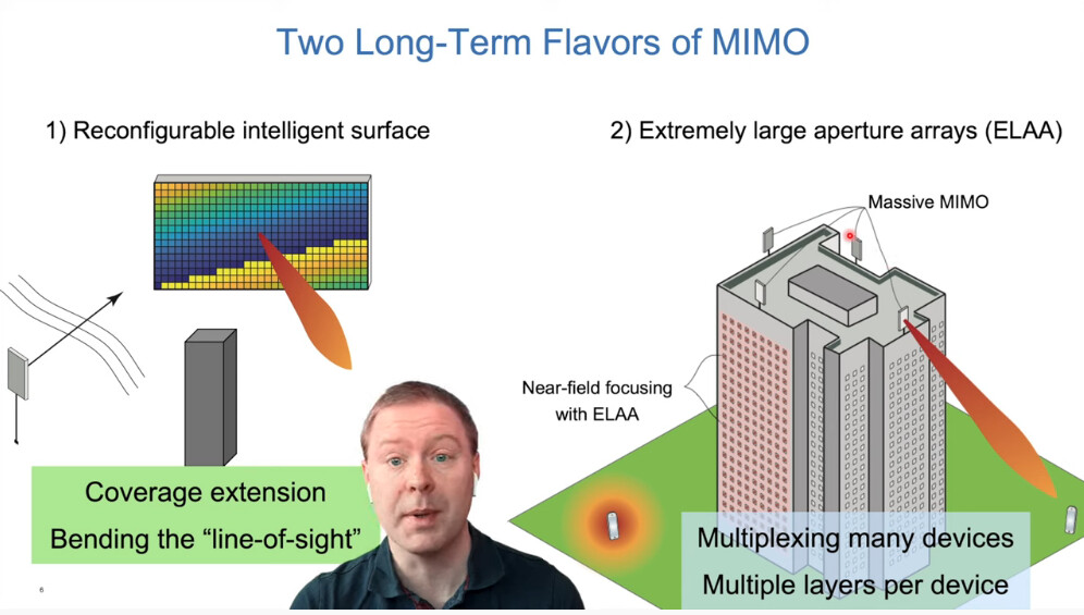
wireless communication mimo antenna array

Highlights

Dimensional Complexity: Scalar channels manage single-dimensional signals, while vector channels handle multi-dimensional signals enhancing capacity.
Noise and Capacity: Both channels use additive Gaussian noise, but capacity calculations differ significantly due to the additional degrees of freedom in vector channels.
Applications in Modern Systems: Scalar channels find use in simple SISO systems, whereas vector channels are integral to MIMO and advanced wireless communication systems.

Introduction

Communication systems rely heavily on the transmission of signals through various channels, where noise and interference can degrade performance. Among the most widely used models are Gaussian channels. These models are pivotal in understanding how noise affects information transmission. In this article, we explore the comparison between scalar and vector Gaussian channels, detailing their operational principles, mathematical representations, capacity formulations, and practical applications in modern communication systems.

Fundamental Concepts

Scalar Gaussian Channels

A scalar Gaussian channel is the simplest model representing a communication channel where the input and output are scalar values. This model assumes that the signal is distorted by additive white Gaussian noise (AWGN). The noise, characterized by its mean and variance, is independent of the transmitted signal. The mathematical representation typically uses the equation:

Mathematical Model

The scalar channel is modeled as:

\( y = x + n \), where \( x \) represents the transmitted signal, \( y \) the received signal, and \( n \) the additive Gaussian noise with variance \( \sigma^2 \).

This model simplifies the analysis of system performance, particularly in terms of calculating the channel capacity, where capacity \( C \) is determined by the signal-to-noise ratio (SNR). The capacity of a scalar channel under an average power constraint \( P \) and noise power \( N \) is given by:

\( C = \frac{1}{2} \log_2\Big(1 + \frac{P}{N}\Big) \).

This equation illustrates the logarithmic relationship between the channel capacity and the power ratio, emphasizing how increased power relative to noise improves channel efficiency.

Vector Gaussian Channels

In contrast to scalar channels, vector Gaussian channels deal with multi-dimensional signals. This channel model is particularly relevant in scenarios where multiple antennas are employed for transmitting and receiving signals, such as in MIMO (Multiple Input Multiple Output) systems.

Mathematical Model and Representation

A vector Gaussian channel can be described by the equation:

\( \mathbf{y} = \mathbf{Hx} + \mathbf{n} \), where:

\( \mathbf{x} \) is the input vector,
\( \mathbf{y} \) is the output vector,
\( \mathbf{H} \) is the channel matrix representing the influence between input and output channels, and
\( \mathbf{n} \) is the Gaussian noise vector which may have correlated elements depending on channel conditions.

The channel capacity in vector Gaussian channels is much more involved, as it requires accounting for the eigenvalues of the channel matrix and optimally allocating power across different dimensions. Techniques such as the waterfilling algorithm are employed to determine the optimal input power distribution across the different channels.

Detailed Comparison

Dimensionality and Signal Processing

The most significant difference between scalar and vector Gaussian channels stems from their dimensionality:

Scalar Channels

Scalar channels involve single-dimensional signal processing. This simplicity makes them easier to analyze and implement. The transmission involves a one-to-one mapping between the transmitted signal and its received counterpart, making them ideal for straightforward scenarios such as point-to-point communications where interference can be managed effectively.

Vector Channels

Vector channels, on the other hand, involve multiple simultaneous transmissions. Here, signals are processed in a multi-dimensional space, which allows the exploitation of spatial diversity. This diversity is a central advantage in modern communication systems, notably improving system robustness and throughput by enabling spatial multiplexing. By leveraging multiple antenna arrays, vector channels can support several parallel data streams.

Noise, Interference, and Signal Separation

Both channel types are influenced by Gaussian noise, but the complexity varies:

Noise Model in Scalar Channels

In scalar channels, the noise is typically modeled as i.i.d. (independent and identically distributed) Gaussian noise. Each signal transmission is perturbed by noise that does not correlate with others. The relative simplicity of this noise model facilitates straightforward capacity calculations and performance evaluations.

Noise Model in Vector Channels

For vector channels, noise is represented by a vector whose components might be correlated. The channel matrix \( \mathbf{H} \) plays a significant role in how noise affects the output. With multiple transmissions, interference among the channels can occur, requiring sophisticated signal processing techniques to decouple individual signals effectively. The “decoupling principle” in vector channels helps isolate each data stream, effectively reducing complex multi-dimensional noise effects to a set of parallel scalar problems.

Capacity Analysis and Formulation

Channel capacity is a measure of the maximum rate of data transfer through a channel under noise constraints.

Scalar Channel Capacity

The capacity of a scalar Gaussian channel is relatively straightforward and is given by:

\( C = \frac{1}{2} \log_2\Big(1 + \frac{P}{N}\Big) \),

where \( P \) is the signal power and \( N \) is the noise power. This relationship is central in demonstrating that increasing the power relative to noise improves the communication capacity logarithmically.

Vector Channel Capacity

The capacity of vector Gaussian channels is determined by the characteristics of the channel matrix \( \mathbf{H} \) and the noise covariance matrix. The calculation involves the spectral decomposition of the matrix to yield eigenvalues that then underpin the optimal power allocation. The capacity is expressed as:

\( C = \max_{\text{power allocation}} \sum_{i=1}^{n} \frac{1}{2}\log_2\Big(1 + \frac{P_i \lambda_i}{N}\Big) \),

where \( \lambda_i \) are the eigenvalues of \( \mathbf{H}^T \mathbf{H} \) and \( P_i \) is the power allocated to the \( i \)-th eigenchannel. This expression demonstrates that vector channels can achieve significantly higher capacities by optimally splitting the available power among multiple eigenchannels.

Applications in Modern Communication Systems

The choice between scalar and vector Gaussian channels greatly influences the design and functionality of communication systems.

Scalar Channels in Practice

Scalar Gaussian channels are typically used in simpler communication systems, such as:

Traditional fixed-point or single-antenna communications.
Applications where signal processing simplicity is a priority.
Systems where cost, complexity, and processing power are strictly limited.

Although these channels are effective under certain conditions, their single-dimensional nature may restrict data throughput and system robustness, particularly in environments with significant interference.

Vector Channels in Modern Wireless Communication

Vector channels are integral to state-of-the-art communication technologies. Their multi-dimensional capabilities allow for:

MIMO Techniques: Exploiting multiple antennas to send and receive several data streams in parallel.
Enhanced Reliability: Utilizing spatial diversity to cope with fading and interference, significantly improving the robustness of the transmitted signal.
Higher Throughput: Achieving greater data rates by optimizing the use of available spectral resources.
Adaptive Signal Processing: Capable of exploiting channel state information to dynamically adjust transmission strategies in response to varying conditions.

These capabilities make vector Gaussian channels essential for modern cellular networks, Wi-Fi systems, and next-generation broadband communication technologies.

Comparative Summary Table

Feature	Scalar Gaussian Channels	Vector Gaussian Channels
Signal Dimensionality	Single Input, Single Output (SISO)	Multiple Inputs, Multiple Outputs (MIMO)
Noise Model	Independent and Identically Distributed Gaussian Noise	Often Correlated Gaussian Noise across Dimensions
Capacity Calculation	\( \frac{1}{2} \log_2(1 + \frac{P}{N}) \)	Involves eigenvalue decomposition and waterfilling strategy: \( \sum_{i=1}^{n} \frac{1}{2}\log_2\Big(1 + \frac{P_i \lambda_i}{N}\Big) \)
Complexity	Low Complexity, Straightforward Implementation	High Complexity, Requires Advanced Signal Processing Techniques
Practical Applications	Basic Communication Systems, SISO Links	Advanced Wireless Systems, MIMO Networks
Multiplexing Capability	Limited, No Spatial Multiplexing	High, Enables Spatial Multiplexing for Increased Data Rates

Practical Considerations in Channel Design

Scalability and Implementation Issues

When designing communication systems, the choice between scalar and vector Gaussian channels depends not only on theoretical capacity but also on real-world implementation challenges. Scalar channels offer simplicity that can be beneficial in systems with strict limits on hardware complexity and power consumption. Their simplicity also affords easier analysis and an easier understanding of the fundamental limits of the channel.

However, in environments where high data rates and robust performance are critical, such as in urban cellular networks or high-speed Wi-Fi, vector channels become indispensable. The ability to use multiple antennas and exploit multiple dimensions allows systems to dynamically adjust to varying signal conditions and interference patterns. This adaptability is key to maximizing the overall network throughput and reliability.

Signal Processing and Decoupling

One of the challenges in vector Gaussian channels is the separation and decoupling of individual data streams. Advanced digital signal processing (DSP) techniques are required to disentangle the signals that are superimposed in the spatial domain. The decoupling principle in vector channels suggests that the optimal estimate of each symbol, when properly processed, achieves performance on par with its scalar counterpart. This insight allows designers to conceptualize complex MIMO systems as a set of parallel scalar channels after suitable processing.

In practical implementations, algorithms that perform channel estimation, equalization, and interference mitigation are critical. The performance of these algorithms directly influences the overall capacity and reliability of the vector Gaussian channel.

Error Performance and Robustness

Error performance is another critical metric in the evaluation of communication channels. Scalar Gaussian channels, while simpler, may be more susceptible to noise and fading since they lack the diversity offered by multiple antennas. In contrast, the inherent diversity in vector channels not only improves capacity but also enhances robustness against selective fading and spatially correlated noise.

Robust adaptive modulation and coding techniques are often deployed in vector channels to further improve performance under adverse conditions. These techniques harness the rich statistical properties of the channel matrix, resulting in improved reliability and lower error rates in high-demand applications.

Advanced Techniques and Theoretical Insights

Waterfilling Algorithm in Vector Channel Capacity

In vector Gaussian channels, one prominent method used for maximizing channel capacity is the waterfilling algorithm. This algorithm optimally allocates power over different eigenchannels based on the channel conditions. The strategy is analogous to filling a set of vessels with water, where each vessel represents an eigenvalue, and power is distributed in a way that the ‘water level’ is kept constant across them.

Spectral Decomposition and Eigenvalue Analysis

The role of spectral decomposition in analyzing vector channels cannot be overstated. By decomposing the channel matrix \( \mathbf{H} \) into its eigenvalues and eigenvectors, engineers obtain critical insights into how best to split the available power. The eigenvalues indicate the strength of each independent channel mode. Subsequently, maximizing individual terms in the capacity summation allows for tailored power allocation strategies tuned to the channel's instantaneous conditions.

The interplay between mathematical theory and practical signal processing techniques forms the backbone of modern wireless system design, offering a clear pathway to achieving the ostensibly high capacities promised by vector channels.