Visualizing Solutions: How to Graph the Linear Inequality \(x + y \leq 200\)

Highlights of Graphing \(x + y \leq 200\)

Identify the Boundary: Start by graphing the line \(x + y = 200\), which divides the coordinate plane into two regions.
Determine the Line Type: Since the inequality includes "equal to" (\(\leq\)), the boundary line is solid, indicating points on the line are part of the solution.
Shade the Solution Area: Use a test point (like the origin) to determine which side of the line satisfies the inequality; shade this region (below the line) to represent all valid \( (x, y) \) pairs.

Understanding the Linear Inequality

What Does \(x + y \leq 200\) Represent?

The inequality \(x + y \leq 200\) is a linear inequality in two variables, \(x\) and \(y\). It doesn't represent a single line but rather a vast region on the coordinate plane. Every point \( (x, y) \) within this region (including its boundary) satisfies the condition that the sum of its x-coordinate and y-coordinate is less than or equal to 200. Graphing this inequality allows us to visualize all possible solutions simultaneously.

This type of inequality is fundamental in various fields, including algebra, economics (budget constraints), and operations research (resource limitations in linear programming).

Step-by-Step Guide to Graphing \(x + y \leq 200\)

Step 1: Graph the Boundary Line

Turning Inequality into Equality

The first step is to treat the inequality as an equation to find the boundary line that separates the coordinate plane. Replace the \(\leq\) sign with an \(=\) sign:

\[ x + y = 200 \]

This is the equation of a straight line.

Finding Key Points: Intercepts

The easiest way to graph a line is often by finding its intercepts (where the line crosses the axes):

Y-intercept (where \(x = 0\)): Substitute \(x = 0\) into the equation: \(0 + y = 200 \implies y = 200\). The y-intercept is at the point \((0, 200)\).
X-intercept (where \(y = 0\)): Substitute \(y = 0\) into the equation: \(x + 0 = 200 \implies x = 200\). The x-intercept is at the point \((200, 0)\).

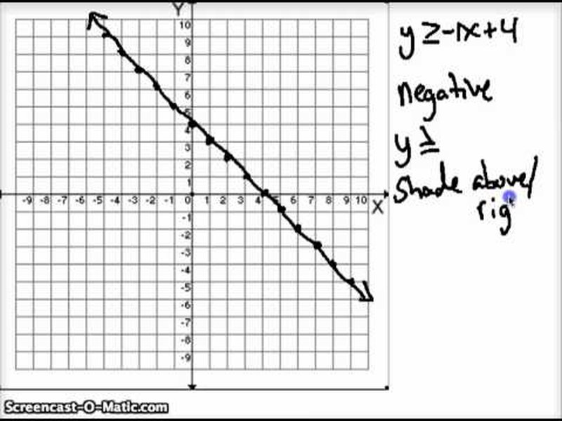
Example of plotting intercepts for a linear equation

Visual representation of finding intercepts to plot a line. While this image shows a different inequality, the concept of using intercepts applies directly to \(x + y = 200\).

Drawing the Line

Plot the two intercepts, \((0, 200)\) and \((200, 0)\), on the coordinate plane. Then, draw a straight line passing through both points. This line represents all pairs \( (x, y) \) for which \(x + y\) is exactly equal to 200.

Alternatively, you can rewrite the equation in slope-intercept form (\(y = mx + b\)):

\[ y = -x + 200 \]

This tells us the slope (\(m\)) is -1 (meaning the line goes down 1 unit for every 1 unit it moves to the right) and the y-intercept (\(b\)) is 200, confirming our point \((0, 200)\).

Step 2: Determine the Line Type (Solid or Dashed)

The type of line depends on the inequality symbol:

For \(\leq\) (less than or equal to) or \(\geq\) (greater than or equal to), the line is solid. This indicates that points *on* the line are included in the solution set.
For \(<\) (less than) or \(>\) (greater than), the line is dashed. This indicates that points *on* the line are *not* part of the solution.

Since our inequality is \(x + y \leq 200\), we use a solid line for \(x + y = 200\).

Step 3: Select the Correct Region (Shading)

Using a Test Point

The line \(x + y = 200\) divides the coordinate plane into two half-planes. We need to determine which half-plane contains the points that satisfy \(x + y \leq 200\). To do this, we select a test point that is *not* on the line. The origin, \((0, 0)\), is usually the easiest choice, provided the line doesn't pass through it.

Substitute the coordinates of the test point \((0, 0)\) into the original inequality:

\[ x + y \leq 200 \] \[ 0 + 0 \leq 200 \] \[ 0 \leq 200 \]

Interpreting the Result

The statement \(0 \leq 200\) is true. This means that the test point \((0, 0)\) *is* part of the solution set. Therefore, we must shade the entire region (half-plane) that contains the origin \((0, 0)\). This is the region below and to the left of the solid line \(x + y = 200\).

If the test point had resulted in a false statement, we would shade the region on the *opposite* side of the line.

Graph showing shaded region for a linear inequality

Example graph illustrating the concept of shading the solution region for a linear inequality. The shaded area represents all points satisfying the inequality.

The Final Graph

The final graph consists of the solid line \(x + y = 200\) and the entire shaded region below and to the left of it. This shaded area represents the infinite set of points \( (x, y) \) for which the sum of the coordinates is less than or equal to 200.

Mindmap Summary: Graphing \(x + y \leq 200\)

Visualizing the Process

This mindmap outlines the key steps and concepts involved in graphing the linear inequality \(x + y \leq 200\). It provides a quick visual summary of the entire process, from identifying the boundary line to determining the final shaded solution region.

mindmap root["Graphing x + y ≤ 200"] id1["Step 1: Boundary Line"] id1a["Equation: x + y = 200"] id1b["Find Intercepts"] id1b1["X-intercept (y=0): (200, 0)"] id1b2["Y-intercept (x=0): (0, 200)"] id1c["Plot Intercepts & Draw Line"] id1d["Alternative: Slope-Intercept Form y = -x + 200"] id2["Step 2: Line Type"] id2a["Inequality: ≤ (or ≥)"] id2b["Result: Solid Line"] id2c["Meaning: Points on the line are solutions"] id3["Step 3: Shading the Region"] id3a["Choose Test Point (not on line)"] id3a1["Example: (0, 0)"] id3b["Substitute into Inequality: 0 + 0 ≤ 200"] id3c["Result: 0 ≤ 200 (True)"] id3d["Shade the side containing the test point"] id3e["Region: Below / Left of the line"] id4["Final Graph"] id4a["Solid line connecting (0, 200) and (200, 0)"] id4b["Shaded area below and including the line"] id5["Context (Optional)"] id5a["Non-negativity: x ≥ 0, y ≥ 0"] id5b["Solution in First Quadrant (Triangle)"] id5c["Applications: Linear Programming, Budget Constraints"]

This visualization helps reinforce the logical flow required to accurately represent the inequality on the coordinate plane.

Key Considerations in Graphing Linear Inequalities

Relative Importance of Steps

When graphing linear inequalities like \(x + y \leq 200\), several steps are crucial. The radar chart below offers an opinionated view on the relative importance or potential difficulty associated with each core aspect of the process. Understanding these nuances helps in avoiding common errors.

This chart highlights that understanding the inequality symbol's meaning (determining line type and shaded region) is often considered the most crucial step, while finding intercepts or slope are fundamental but perhaps less prone to conceptual errors once the method is known.

Verifying Points in the Solution Set

Testing Example Coordinates

To confirm our understanding, let's test a few points to see if they fall within the solution region defined by \(x + y \leq 200\).

Point (x, y)	Calculation (x + y)	Is \(x + y \leq 200\)?	Location Relative to Line	In Solution Set?
(50, 100)	50 + 100 = 150	150 ≤ 200 (True)	Below	Yes
(0, 0)	0 + 0 = 0	0 ≤ 200 (True)	Below	Yes
(100, 100)	100 + 100 = 200	200 ≤ 200 (True)	On the line	Yes
(200, 0)	200 + 0 = 200	200 ≤ 200 (True)	On the line	Yes
(-50, 100)	-50 + 100 = 50	50 ≤ 200 (True)	Below	Yes
(150, 100)	150 + 100 = 250	250 ≤ 200 (False)	Above	No
(200, 50)	200 + 50 = 250	250 ≤ 200 (False)	Above	No

This table clearly shows that points on the line or in the region below/left of the line satisfy the inequality, while points above/right do not.

Visual Demonstration: Graphing Constraints

Graphing Inequalities in Linear Programming

Inequalities like \(x + y \leq 200\) are often used as constraints in linear programming problems, where we aim to optimize an objective function subject to certain limitations. Understanding how to graph these constraints is a crucial first step. The video below provides a tutorial on drawing constraints on a graph, which is directly applicable to our inequality.

This video demonstrates the process for various constraints, reinforcing the techniques discussed: finding intercepts, drawing the boundary line (solid or dashed), and identifying the feasible region (the area satisfying all constraints, analogous to our single shaded region).

Frequently Asked Questions (FAQ)

Why do we use a test point like (0, 0)? +

What if the inequality was \(x + y < 200\)? +

What if the test point (0, 0) is on the line? +

What if \(x\) and \(y\) must be non-negative? +