Unveiling the Intricacies of High NA Parabolic Mirror Simulations

Explore how beam modes, mirror design, and optical parameters converge in advanced electromagnetic simulations

Key Insights

Vectorial Field Simulation: Accurately modeling the electromagnetic fields requires vectorial treatments, especially for high NA conditions.
Detailed Geometrical Parameters: Mirror diameter, depth, focal length, and the input beam's spatial mode significantly influence the focal spot distribution.
Advanced Simulation Tools: Software such as COMSOL, Meep, and VirtualLab can handle complex boundary conditions and offer flexibility with modeling setups.

Simulation Overview

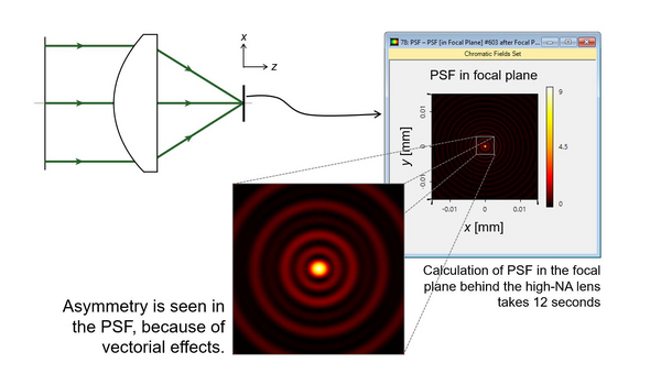
Simulating the electromagnetic field distribution at the focus of a high numerical aperture (NA) parabolic mirror is an intricate process that involves several key considerations. A high NA parabolic mirror, due to its ability to gather and concentrate light to extremely small spot sizes, necessitates a full vectorial treatment of the fields rather than relying on scalar approximations. It is crucial to simulate the fields accurately as these significantly depend on both the mirror geometry (diameter, depth, and focal length) and the spatial mode properties of the incoming collimated optical beam.

The simulation process typically involves defining the incoming beam characteristics, modeling the mirror geometry through the parabolic equation \( \[ y = \frac{x^2}{4f} \] \) (where \( \text{\( f \)} \) is the focal length), and using computational techniques to resolve the electromagnetic field distribution in the focal region. The spatial mode of the beam – whether it is TEM00, radially polarized, or another mode – plays a significant role in the interference patterns and focusing properties observed.

Core Simulation Components

1. Defining Optical Beam Parameters

Spatial Mode and Polarization

The incoming optical beam’s spatial mode (e.g., Gaussian, flat-top, or higher-order mode) is essential in determining the distribution of the electric field in the focal area. Particular polarization, such as linear or radially polarized light, produces different focal spot characteristics. For instance, radially polarized beams have been shown to produce a strong longitudinal field component, which may lead to tighter focusing and is advantageous in applications like tip-enhanced spectroscopy.

Wavelength and Intensity

Parameters such as the wavelength and beam waist determine diffraction effects and the focusing capabilities. These properties must be incorporated into the simulation to accurately predict the field distribution.

2. Mirror Geometry

Mirror Diameter, Depth, and Focal Length

The parabolic mirror's physical dimensions are critical. The diameter influences the numerical aperture and the amount of light collected, while the depth and focal length define the parabolic shape. This mirror shape is mathematically described as:

\( \[ y = \frac{x^2}{4f} \] \)

Where a precise focal point is determined by the mirror's depth and curvature, ensuring that the incoming collimated beam is focused as accurately as possible. High NA conditions may result in aperture angles approaching or exceeding 90 degrees, further complicating the electromagnetic interactions.

3. Numerical Aperture (NA) and Vectorial Effects

High NA Considerations

When dealing with high NA systems, scalar diffraction theories become insufficient. A full vectorial treatment, often employing the Debye integral method or similar approaches, must be used. This treatment calculates the electric field components and their interference in the highly converging beam. Such simulations capture the effects of polarization and phase variations across the wavefront.

4. Simulation Software and Techniques

Software Tools

There are several software options available for these complex simulations:

COMSOL Multiphysics: Suitable for finite element analysis (FEA) where meshing of the parabolic surface and electromagnetic fields occurs. It can handle boundary conditions and incorporate materials' properties.
Meep: An open-source tool based on the finite-difference time-domain (FDTD) method. It is particularly useful for computing time-evolution of the electromagnetic fields over a defined spatial grid.
VirtualLab: Implements fast physical-optics simulation techniques that are effective for high NA focusing, incorporating detailed beam mode and mirror geometry specifics.
MATLAB: Often used for custom simulations and to provide flexible scripting that can integrate various simulation steps and mathematical modeling.

Simulation Approaches

Two primary methodologies can be employed:

Full Vectorial Treatment: This approach involves solving Maxwell's equations directly through numerical methods that take into account the polarization and amplitude variations across the incoming beam. Methods like the Debye integral, modified for vector fields, are central in this approach.
Finite Difference Time Domain (FDTD): An efficient time-domain method that discretizes the FDTD algorithm on a spatial grid, allowing the simulation to compute the evolution of electromagnetic fields and their interactions. This is particularly useful when simulating non-trivial geometries.

Parameter Integration and Analysis

Creating a Comprehensive Simulation Model

The simulation process begins by integrating the optical beam parameters with the geometrical attributes of the parabolic mirror. Given that these components strongly interact, it is beneficial to outline the parameters in a table format to ensure clarity during the simulation setup.

Parameter	Description	Importance
Beam Spatial Mode	Gaussian, TEM00, Radially polarized, etc.	Determines focal interference patterns and field distribution.
Wavelength	Optical wavelength of the beam (nm or μm)	Impacts diffraction and focal spot size.
Numerical Aperture (NA)	Defined by mirror geometry and beam angle.	Critical for determining focusing properties and field distribution.
Mirror Diameter	Size of the parabolic mirror, influencing light collection.	Affects intensity and resolution at the focal point.
Mirror Depth	Depth relates to the curvature of the mirror.	Determines how the beam is redirected towards the focal point.
Focal Length (f)	Focus distance from the mirror vertex to the focal point.	Central to the parabolic equation and overall focusing performance.

Implementation Details

Practical Steps for Simulation

Step 1: Define the Simulation Domain

Begin by establishing your simulation domain. This involves setting up a three-dimensional space that encompasses the entire mirror along with sufficient surrounding space to accurately compute the incoming beam’s interactions and the subsequent field focus.

In software like COMSOL or Meep, you will define boundary conditions. Perfectly Matched Layers (PMLs) are utilized to minimize reflections from the edges of the simulation domain, ensuring that the calculation only captures the true behavior of the incident and focused beam.

Step 2: Model the Parabolic Mirror

Utilize the parabolic equation \( \[ y = \frac{x^2}{4f} \] \) to generate the mirror profile. The geometry must be created with high precision: the mirror diameter defines the aperture, while the depth influences how much the surface deviates from a flat plane. An accurate model of the mirror is essential for capturing the correct phase shifts and reflection properties.

The mirror's surface might be discretized into small elements (using a meshing strategy), particularly when using FDTD or finite element methods, so that the vectorial boundary conditions at the mirror’s surface are rigorously applied.

Step 3: Input Beam Characteristics

Incorporate the spatial mode of the collimated optical beam. This includes specifying the wavelength, beam waist, and polarization state. For example, if the beam is radially polarized, this aspect should be detailed in the simulation parameters to capture the distinct focal properties such as enhanced longitudinal electric fields.

Numerical input must ensure that the phase front is modeled correctly, as deviations can significantly alter the focal spot distribution.

Step 4: Run the Simulation and Analyze Results

After setting up the geometry, defining the input beam, and setting the simulation conditions (such as the time step and spatial grid resolution), run the simulation. Advanced visualization tools within the simulation software allow you to inspect the resulting intensity distributions and vector electric field components in the focal plane. The simulation output should provide insights into the spot size, shape, and potential aberrations induced by the mirror geometry.

It is important to iterate over the simulation parameters – adjusting mirror depth, diameter, and focal length – to understand how modifications affect the field distribution at focus. This iterative approach is crucial especially in experimental setups and prototype validations.

Examples of Simulation Approaches

Finite Difference Time Domain (FDTD) Method

The FDTD method discretizes both time and space and is particularly useful for handling complex optical systems with non-analytic boundaries. When using FDTD, you need to consider stability conditions (e.g., Courant conditions) and ensure that the meshing is fine enough to resolve the variations in the electromagnetic field.

Software tools like Meep provide a robust platform for FDTD simulations by allowing you to define materials, specify the spatial mode of the light source, and calculate the evolution of electric and magnetic fields over time.

Debye Integral and Vectorial Approaches

The Debye integral approach, especially in its 3D vectorial version, is effective when modeling the intense focusing achieved by high NA mirrors. This method takes into account the contributions of all elementary wavelets emanating from the mirror surface, offering a holistic view of how the fields overlap and interfere at the focus.

Accurate computation using the Debye integral requires numerical integration over the mirror's aperture, considering the distribution of phase and amplitude. This method is therefore computationally demanding but provides higher fidelity for systems where the vector nature of light significantly influences the behavior.

Integrating Simulation Results

Data Analysis and Visualization

Upon completion of the simulation, focus your analysis on key parameters:

Intensity distribution and spot size at the focus.
Electric field vectors and polarization distribution.
Phase and amplitude variations across the focal plane.

Modern simulation platforms offer advanced visualization modules that can help identify potential aberrations. By comparing different configurations (for example, altering the mirror’s depth or the beam’s polarization), you can fine-tune the design to optimize focusing performance.

Practical Implementation: Example Simulation Code

Basic FDTD Pseudocode Example

The example below illustrates an FDTD approach using Python. While it is a simplified version, it outlines the key steps – discretizing the simulation domain, applying boundary conditions, and updating the electric field:


# Import necessary libraries
import numpy as np
import matplotlib.pyplot as plt

# Simulation parameters
Nx, Nt = 1000, 500
L = 1.0                        # Length of the simulation domain
dx = L / (Nx - 1)
c = 3e8                        # Speed of light in vacuum
dt = dx / (2 * c)              # Time step using Courant condition

# Initialize the electric field array
Ex = np.zeros((Nx, Nt))

# Define a Gaussian beam as input
x = np.linspace(0, L, Nx)
Ex[:, 0] = np.exp(-((x - L/2)**2) / (0.01))

# FDTD loop
for n in range(0, Nt - 1):
    for i in range(1, Nx - 1):
        Ex[i, n+1] = Ex[i, n] + (c * dt / dx) * (Ex[i+1, n] - Ex[i-1, n])

# Visualize the final field distribution
plt.imshow(Ex.T, aspect='auto', cmap='jet')
plt.title("Electric Field Distribution")
plt.xlabel("Spatial Index")
plt.ylabel("Time Step")
plt.colorbar()
plt.show()

This pseudocode demonstrates the basic principles. For accurate optical simulations involving parabolic mirrors and high NA conditions, consider using established simulation tools like Meep or COMSOL which can manage full vectorial treatments and boundary complexities.

Application Areas and Further Studies

Implications in Modern Optical Applications

High NA parabolic mirrors and their electromagnetic field distribution simulations are pivotal in a wide array of applications:

Confocal Microscopy: Enhanced resolution and field exposure for medical imaging and material science.
Particle Acceleration: Utilizing focused beams with strong longitudinal fields for precise particle control.
Tip-Enhanced Raman Spectroscopy (TERS): Enabling sub-diffraction imaging by leveraging the tight focal spots.
Digital Holography: Achieving high-fidelity reconstructions based on interference patterns formed at the focus.

The iterative simulation process can help optimize these applications, allowing for tailored designs that meet specific operational criteria. Fine-tuning simulation parameters such as the beam mode and mirror geometry can lead to breakthroughs in precision focusing and imaging technologies.