Taming Your KAN: Why Your [0,1] Output Transformation Might Be Fueling Overfitting (and How to Fix It)

Unlock stable Kolmogorov-Arnold Network performance by addressing output distribution shifts and mitigating overfitting effectively.

You're encountering a common yet tricky challenge with Kolmogorov-Arnold Networks (KANs). While adapting KANs for tasks requiring outputs constrained between 0 and 1, you've rightly observed that different transformation methods (like Sigmoid, scaled Tanh, or even sophisticated approaches using Beta distributions parameterized by Softplus outputs) drastically alter the distribution of the KAN layer's final activations. Your suspicion that this distribution instability contributes to model overfitting is astute. Let's delve into why this happens and explore robust strategies to achieve a more stable output distribution and significantly reduce overfitting.

Essential Insights: Stabilizing KAN Outputs

Focus Beyond the Final Function: While the [0, 1] transformation matters, overfitting in KANs often stems more fundamentally from their high flexibility and complexity (learnable spline activations on edges) rather than the final output function alone.
Normalize Before Transforming: A crucial step is to stabilize the raw output distribution *from* the KAN layer *before* applying your chosen [0, 1] mapping function. Techniques like batch normalization can make the final transformation less disruptive.
Combine Multiple Strategies: Effectively tackling overfitting requires a multi-pronged approach, combining output stabilization with robust regularization techniques (like L1/L2, KAN-specific sparsification), model complexity control, and sound training practices (like early stopping).

Understanding KANs and the Output Distribution Dilemma

Why KANs Behave Differently

Unlike traditional Multi-Layer Perceptrons (MLPs) that use fixed activation functions (like ReLU or Sigmoid) at the nodes, KANs place *learnable* activation functions on the *edges* connecting nodes. These are often parameterized as splines (piecewise polynomials), allowing the network to learn highly complex and adaptive non-linear relationships directly from data. This architectural difference grants KANs significant expressive power but also makes them inherently more complex and potentially sensitive to training data specifics.

The Transformation Tango: Impact on Distribution

When you take the raw, potentially unbounded output of a KAN layer and force it into the [0, 1] range using a non-linear function (Sigmoid, Tanh, etc.), you are fundamentally reshaping its distribution. Consider these examples:

Sigmoid: Compresses the entire real number line into (0, 1), but values far from zero get squashed near 0 or 1, potentially leading to vanishing gradients (saturation).
Scaled Tanh \( \frac{\tanh(x) + 1}{2} \): Also maps to (0, 1) but exhibits similar saturation behavior for large positive or negative inputs.
Beta Distribution (via Softplus): This is more sophisticated. Using Softplus ensures the parameters \( \alpha \) and \( \beta \) are positive, and the Beta distribution's mean inherently lies in [0, 1]. However, the relationship between the KAN output and the resulting mean is complex and depends heavily on the learned \( \alpha \) and \( \beta \). Small changes in the KAN output could lead to significant shifts in the mean's location and the distribution's shape (variance, skewness).
Custom Functions (e.g., \(1 - \exp(-x^2)\)): These map to [0, 1) but might introduce unusual gradient behavior or arbitrarily restrict the KAN's learned representation, potentially hindering generalization.

The problem arises because the KAN layer learns its spline functions based on the gradients flowing back through this final transformation. If the transformation causes instability or drastically different distributions depending on the input batch, it can confuse the learning process, making the KAN latch onto noise or specific artifacts in the training data – a hallmark of overfitting.

Strategies for a More Stable and "Appropriate" Output Distribution

1. Normalize the KAN Output First!

Perhaps the most impactful single change is to normalize the raw output of the KAN layer *before* applying the final [0, 1] transformation. This helps ensure the input to your Sigmoid, Tanh, or Beta parameterization function has a more consistent scale and distribution (e.g., zero mean, unit variance) across different batches, making the final transformation's effect less erratic.

Techniques for Normalization:

Batch Normalization: Apply a standard Batch Normalization layer after the KAN layer.
Layer Normalization: Similar to Batch Norm but normalizes across features for a single data point, sometimes preferred for varying batch sizes or RNN-like structures.
Simple Standardization: Manually subtract the batch mean and divide by the batch standard deviation.

Example Implementation Snippet:

Consider modifying your forward pass like this:


import torch
import torch.nn as nn

# Assume self.kan is your KAN layer and self.final_activation is your chosen [0,1] function (e.g., Sigmoid)
# Option 1: Using nn.BatchNorm1d (if output is suitable shape)
# self.bn = nn.BatchNorm1d(num_features=output_dim_of_kan) 
# def forward(self, inputx):
#     x_raw = self.kan(inputx)
#     # Ensure shape is compatible with BatchNorm1d, e.g., (batch_size, features)
#     if x_raw.ndim == 1: x_raw = x_raw.unsqueeze(0) # Handle single sample case
#     if x_raw.ndim > 2: x_raw = x_raw.view(x_raw.size(0), -1) # Flatten features if needed
#     x_norm = self.bn(x_raw)
#     x_final = self.final_activation(x_norm)
#     return x_final

# Option 2: Simple Manual Batch Standardization
def forward(self, inputx):
    x_raw = self.kan(inputx) # Raw KAN output, shape e.g., [batch_size, output_dim]
    
    # Normalize across the batch for each feature dimension
    if x_raw.size(0) > 1: # Avoid division by zero for batch size 1
        mean = x_raw.mean(dim=0, keepdim=True)
        std = x_raw.std(dim=0, keepdim=True)
        x_norm = (x_raw - mean) / (std + 1e-6) # Add epsilon for stability
    else:
        x_norm = x_raw # Or apply instance normalization if needed

    # Apply final activation to normalized output
    # Example using Sigmoid:
    x_final = torch.sigmoid(x_norm) 
    
    # Example using Beta distribution (assuming x_norm has 2 features for alpha, beta):
    # eps = torch.finfo(x_norm.dtype).eps
    # alpha = F.softplus(x_norm[...,0]).clamp(min=eps) 
    # beta  = F.softplus(x_norm[...,1]).clamp(min=eps)
    # dist = torch.distributions.Beta(alpha, beta)
    # y_final = dist.mean
    
    return x_final # or y_final if using Beta

Note: Choose the normalization method and implementation details appropriate for your specific model architecture and data flow. Remember to handle potential division by zero with small batches or zero variance.

2. Choosing the Right [0, 1] Transformation

With normalization in place, the choice of the final function becomes less critical for stability, but still influences the output characteristics:

Comparing Common Transformations

The following table summarizes the properties of the transformations you've considered. Remember that normalization prior to these functions generally improves their behavior.

Transformation	Range Guarantee	Gradient Behavior	Distribution Impact	Interpretability	Complexity
Sigmoid: \( \sigma(x) \)	(0, 1)	Vanishes for large \|x\| (Saturation)	Compresses values, can skew towards 0 or 1	Common for probabilities	Low
Scaled Tanh: \( \frac{\tanh(x) + 1}{2} \)	(0, 1)	Vanishes for large \|x\| (Saturation)	Similar to Sigmoid, slightly different shape	Standard alternative	Low
Beta Mean (via Softplus): \( \frac{\alpha}{\alpha+\beta} \)	[0, 1] (Theoretically)	Depends on \( \alpha, \beta \); potentially complex	Explicitly models output as mean of a distribution; shape controllable via \( \alpha, \beta \)	High (if output is a rate/proportion)	Medium (requires 2 outputs, Softplus, clamping)
Custom \( 1 - \exp(-x^2) \)	[0, 1)	Zero gradient at x=0; non-standard	Symmetric around 0; strongly maps values near 0 to values near 0	Low (unless specific physical meaning)	Low

Recommendations:

For general purposes, Normalized Output + Sigmoid or Normalized Output + Scaled Tanh are robust starting points.
If your output naturally represents a rate, proportion, or probability derived from underlying counts or evidence, the Normalized Output + Beta Distribution approach is semantically meaningful and worth refining (ensure stable positive \( \alpha, \beta \) via Softplus and careful clamping/epsilon addition).
Avoid overly specific or non-standard custom functions unless they have strong theoretical justification for your problem, as they might hinder learning or generalization.

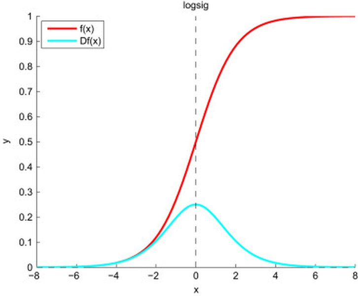
Comparison of bounded activation functions

Visual comparison of different bounded activation functions, illustrating how they shape output. Normalization helps stabilize the input to such functions.

Tackling Overfitting Directly in KANs

Beyond stabilizing the output, directly addressing the KAN's complexity is crucial for preventing overfitting.

1. Regularization Techniques

Standard Methods Adapted for KANs:

L1/L2 Weight Decay: Apply L1 (Lasso) or L2 (Ridge) regularization to the parameters of the learnable spline functions within the KAN layers. L1 encourages sparsity (setting some spline coefficients to zero), potentially simplifying the learned functions.
Dropout: While typically applied to nodes in MLPs, Dropout can be adapted. Consider applying it to the *inputs* or *outputs* of KAN layers, or potentially exploring methods to randomly drop segments or basis functions within the splines during training.

KAN-Specific Regularization:

Sparsification: KANs often benefit from explicit sparsification techniques. Libraries like pykan allow controlling this via a parameter (e.g., lamb in model.train(lamb=0.01)). This encourages the network to use fewer active spline functions or simpler functions, promoting interpretability and reducing overfitting by limiting complexity.
Entropy Regularization: Some research explores regularizing the "entropy" of the activations or gating coefficients to encourage simpler representations.

2. Controlling Model Complexity

Reduce Network Size: Use fewer KAN layers or fewer nodes per layer. Research suggests smaller KANs can achieve comparable performance to larger MLPs.
Simplify Splines: Reduce the complexity of the learnable activation functions by using fewer spline segments (lower grid size in pykan) or lower-order splines (e.g., linear instead of cubic).
Grid Extension Caution: While dynamically increasing the spline grid resolution (grid_update_num in pykan) can improve accuracy, it also significantly increases complexity and the risk of overfitting. Use it cautiously, potentially combined with stronger regularization or early stopping.

3. Data and Training Practices

Increase Data / Augmentation: More diverse training data is one of the most effective ways to improve generalization and reduce overfitting. Use data augmentation techniques relevant to your data type.
Early Stopping: Monitor performance on a separate validation set during training. Stop training when validation performance begins to degrade, even if training performance is still improving. This prevents the model from overfitting to the training set.
Hyperparameter Tuning: Carefully tune learning rates, batch sizes, and optimizer parameters. Smaller batch sizes can sometimes introduce noise that acts as a regularizer.
Ensemble Methods: Train multiple KAN models (perhaps with different initializations or hyperparameters) and average their predictions. This often improves robustness and reduces overfitting compared to a single model.

Visualizing KAN Optimization Strategies

Strategy Effectiveness Radar

This chart provides a conceptual overview comparing different techniques for stabilizing KAN outputs and reducing overfitting. Scores are illustrative (higher is generally better, minimum axis value is 2), reflecting common trade-offs based on the synthesis of information.

Mindmap of Solutions

This mindmap illustrates the interconnected concepts and solutions discussed for managing KAN output distributions and overfitting.

mindmap root["Optimizing KAN Output & Reducing Overfitting"] id1["KAN Characteristics"] id1a["Learnable Edge Activations (Splines)"] id1b["High Expressive Power"] id1c["Potential Complexity"] id2["Problem: Output [0,1] & Overfitting"] id2a["Need for Bounded Output [0,1]"] id2b["Transformation Affects Distribution"] id2b1["Sigmoid/Tanh Saturation"] id2b2["Beta Dist. Complexity"] id2b3["Custom Func. Risks"] id2c["Link to Overfitting"] id2c1["Model Fits Noise"] id2c2["Unstable Gradients"] id3["Solutions: Stabilize & Regularize"] id3a["Stabilize Output Distribution"] id3a1["Normalize KAN Output FIRST"] id3a1a["Batch Norm"] id3a1b["Layer Norm"] id3a1c["Manual Scaling"] id3a2["Choose Final [0,1] Function Wisely"] id3a2a["Sigmoid (Post-Norm)"] id3a2b["Scaled Tanh (Post-Norm)"] id3a2c["Beta Distribution (Post-Norm)"] id3a2d["Avoid Risky Custom Functions"] id3b["Reduce Overfitting Directly"] id3b1["Regularization"] id3b1a["L1/L2 on Splines"] id3b1b["Dropout (Adapted)"] id3b1c["KAN Sparsification (lamb)"] id3b2["Control Complexity"] id3b2a["Reduce Layers/Nodes"] id3b2b["Simplify Splines (grid, order)"] id3b2c["Caution with Grid Extension"] id3b3["Data & Training"] id3b3a["More Data / Augmentation"] id3b3b["Early Stopping"] id3b3c["Hyperparameter Tuning"] id3b4["Advanced"] id3b4a["Ensembles"]

Understanding KAN Mechanics Further

Deep Dive into KAN Concepts

To better grasp how techniques like spline manipulation and sparsification work within KANs, understanding their fundamental principles is helpful. KANs replace the linear transformations and fixed activations of MLPs with learnable spline functions on the network edges. This allows the network to adaptively capture complex patterns. Concepts like B-splines (the building blocks of the learnable functions), grid extension (refining the splines during training), and sparsification (pruning less important spline components) are central to KANs' operation and performance tuning. The following video provides a detailed explanation of the original KAN paper, covering these core ideas.

Understanding these mechanics empowers you to apply techniques like sparsification more effectively, knowing you are simplifying the learned functions to combat overfitting while potentially improving interpretability.

Frequently Asked Questions (FAQ)

Why is normalizing the KAN output before the final [0, 1] function so important? ▼

Normalizing the raw KAN output (e.g., to have zero mean and unit variance across a batch) ensures that the input fed into the final [0, 1] activation function (like Sigmoid or Tanh) has a consistent scale and distribution. Without normalization, the raw outputs might vary wildly in range depending on the input batch, causing the final activation to operate in different regimes (e.g., saturated vs. linear). This inconsistency can destabilize training, make learning difficult, and amplify the distribution shifts you observed, contributing to overfitting. Normalization provides a more stable foundation for the final transformation.

What is KAN Sparsification and how does it help with overfitting? ▼

KAN Sparsification refers to techniques that encourage the network to use fewer "active" components in its learnable spline activation functions or even prune entire connections. This is often achieved by adding a regularization term (controlled by a parameter like `lamb` in `pykan`) during training that penalizes complexity. By forcing the KAN to achieve its goal with simpler or fewer functions, sparsification acts as a form of regularization. It reduces the model's effective number of parameters and its capacity to fit noise in the training data, thereby lowering the risk of overfitting and potentially improving interpretability.

Should I use Sigmoid, Scaled Tanh, or the Beta distribution method for my [0, 1] output? ▼

The best choice depends on your specific task and the semantic meaning of the output:

Use **Sigmoid** or **Scaled Tanh** (after normalizing the KAN output) as robust general-purpose choices if you simply need a value between 0 and 1 without a strong distributional interpretation.
Use the **Beta distribution** approach (parameterizing \( \alpha, \beta \) via Softplus applied to normalized KAN outputs) if your output genuinely represents a probability, rate, or proportion derived from underlying phenomena. It offers more distributional flexibility and interpretability in such cases but is more complex to implement correctly (ensure \( \alpha, \beta > 0 \)).

Always prioritize normalizing the KAN output *before* any of these functions.

Can I apply standard Dropout directly to a KAN? ▼

Applying standard Dropout (which randomly zeros entire node activations) might be possible by placing Dropout layers *before* or *after* KAN layers, treating the KAN layer as a block. However, the effectiveness compared to Dropout in MLPs might differ because KANs learn functions on edges. Some research might explore more integrated forms of Dropout for KANs, like dropping spline basis functions or segments randomly. Applying Dropout to the inputs/outputs of KAN layers is a reasonable starting point for experimentation.

Besides the final transformation, what's the main cause of overfitting in KANs? ▼

The main cause of overfitting in KANs is their inherent **complexity and flexibility**. The learnable spline activation functions on the edges give KANs a very high capacity to model intricate functions. If the training data is noisy or limited, this high capacity allows the KAN to learn the noise and specific artifacts of the training set instead of the underlying general patterns. Techniques like grid extension, while improving potential accuracy, further increase this complexity. Therefore, controlling this complexity via regularization (L1/L2, sparsification), reducing model size (layers, nodes, spline parameters), and using sufficient data with proper training procedures (like early stopping) are crucial to prevent overfitting.