
Unlock Data Insights: Your Step-by-Step Guide to Autoencoders with Keras
Master feature extraction and clustering using neural networks for powerful unsupervised learning.
Highlights
- Master the Workflow: Learn the complete pipeline from setting up your environment and preparing data to building, training, and evaluating an autoencoder using Keras.
- Feature Extraction Power: Discover how autoencoders compress data into meaningful low-dimensional representations (latent features) ideal for downstream tasks like clustering.
- Practical Implementation: Follow clear Python code examples using standard libraries like Pandas, NumPy, Scikit-learn, and Keras (TensorFlow backend) for each step.
Understanding Autoencoders
Autoencoders are a fascinating type of artificial neural network used primarily for unsupervised learning tasks. Their core idea is simple yet powerful: learn a compressed representation (encoding) of input data and then reconstruct the original data from this compressed version (decoding). The goal isn't perfect reconstruction per se, but rather to force the network to learn the most salient features of the data within the compressed representation, often called the "bottleneck" or "latent space".
This process effectively acts as a form of dimensionality reduction and feature extraction. By training the network to minimize the difference between the original input and the reconstructed output (reconstruction error), the encoder learns to capture the essential patterns and discard noise. These learned latent features can then be incredibly useful for various tasks, including anomaly detection (anomalies often have high reconstruction errors), data denoising, and, as we'll explore here, clustering.
Step 1: Setup - Preparing Your Environment
Importing Necessary Libraries
Before we begin, we need to import the essential Python libraries. We'll use Pandas for data handling, NumPy for numerical operations, Scikit-learn for preprocessing and clustering metrics, and Keras (typically using the TensorFlow backend) for building and training our neural network.
# Data Manipulation
import pandas as pd
import numpy as np

# Preprocessing and Evaluation Metrics
from sklearn.model_selection import train_test_split
from sklearn.preprocessing import StandardScaler
from sklearn.metrics import silhouette_score, mean_squared_error

# Clustering
from sklearn.cluster import KMeans

# Dimensionality Reduction for Visualization
from sklearn.decomposition import PCA
from sklearn.manifold import TSNE

# Deep Learning Framework (Keras with TensorFlow backend)
import tensorflow as tf
from tensorflow.keras.models import Model
from tensorflow.keras.layers import Input, Dense
from tensorflow.keras.callbacks import EarlyStopping
from tensorflow.keras.optimizers import Adam

# Plotting
import matplotlib.pyplot as plt

print("Libraries imported successfully!")
Step 2: Data Preparation - Laying the Foundation
Loading and Cleaning the Dataset
The quality of your data significantly impacts the performance of the autoencoder. Start by loading your dataset using Pandas.
# Load your dataset (replace 'your_dataset.csv' with your file path)
try:
    data = pd.read_csv('your_dataset.csv')
    print("Dataset loaded successfully.")
    print("Original data shape:", data.shape)
except FileNotFoundError:
    print("Error: 'your_dataset.csv' not found. Please provide the correct path.")
    # As a placeholder, let's create some dummy data
    print("Creating dummy data for demonstration.")
    data = pd.DataFrame(np.random.rand(500, 10), columns=[f'feature_{i}' for i in range(10)])
    data['target_column'] = np.random.randint(0, 2, 500) # Example target column (optional)

# Display first few rows
print(data.head())

# Handle Missing Values (Example: Dropping rows with any NaN values)
# More sophisticated methods like imputation (e.g., using SimpleImputer) might be better depending on the dataset.
initial_rows = data.shape[0]
data.dropna(inplace=True)
print(f"Removed {initial_rows - data.shape[0]} rows with missing values.")
print("Data shape after handling missing values:", data.shape)

# Separate features (X) and potentially target (y) if it exists and needed for stratified split
# If your dataset is purely for unsupervised learning, you might not have a 'target_column'.
if 'target_column' in data.columns:
    X = data.drop('target_column', axis=1)
    y = data['target_column'] # Keep y for potential stratified splitting, even if not used in training AE
    print("Features (X) and target (y) separated.")
else:
    X = data
    y = None # No target column
    print("Features (X) separated. No target column found.")
Normalization and Data Splitting
Neural networks generally perform better with normalized data. We'll use `StandardScaler` to scale features to have zero mean and unit variance. Then, we split the data into training and testing sets to evaluate the model's generalization ability.
# Normalize the features
scaler = StandardScaler()
X_scaled = scaler.fit_transform(X)
print("Data normalized using StandardScaler.")
print("Scaled data shape:", X_scaled.shape)

# Split the data into training and testing sets
# Use stratify=y if you have a target variable and want to maintain class proportions
# If y is None, remove the stratify argument.
test_size = 0.2
random_state = 42
if y is not None:
    X_train, X_test, y_train, y_test = train_test_split(
        X_scaled, y, test_size=test_size, random_state=random_state, stratify=y
    )
    print(f"Data split into training ({1-test_size:.0%}) and testing ({test_size:.0%}) sets (stratified).")
else:
    X_train, X_test = train_test_split(
        X_scaled, test_size=test_size, random_state=random_state
    )
    y_train, y_test = None, None # Ensure these are None if no target exists
    print(f"Data split into training ({1-test_size:.0%}) and testing ({test_size:.0%}) sets.")

print("Training data shape:", X_train.shape)
print("Testing data shape:", X_test.shape)
Step 3: Building the Autoencoder - Designing the Network
Defining the Encoder, Decoder, and Bottleneck
The autoencoder architecture consists of two main parts:
- Encoder: Compresses the input into a lower-dimensional latent representation. It typically consists of several layers that progressively reduce the dimensionality.
- Decoder: Reconstructs the original input from the latent representation. Its architecture usually mirrors the encoder's but in reverse, progressively increasing dimensionality.
The layer with the smallest dimensionality between the encoder and decoder is the "bottleneck", holding the compressed representation.
Activation Functions
We'll use the Rectified Linear Unit (ReLU) activation function for the hidden layers in both the encoder and decoder. ReLU is computationally efficient and helps mitigate the vanishing gradient problem. For the final output layer of the decoder, we'll use the Sigmoid activation function. Since our input data was scaled (typically between roughly -3 and +3 after StandardScaler, though not strictly bounded), Sigmoid (outputting values between 0 and 1) might not be the perfect choice if aiming for exact reconstruction of scaled values. However, it's commonly used in examples, assuming the goal is more about capturing structure than precise value reconstruction, or if inputs were initially scaled to [0, 1]. A linear activation might be theoretically better for reconstructing standardized data, but Sigmoid often works in practice for learning representations.
# Define model parameters
input_dim = X_train.shape[1]  # Number of features
encoding_dim = 32 # Size of the bottleneck layer (hyperparameter)

# --- Encoder ---
input_layer = Input(shape=(input_dim,), name='Input_Layer')
# Hidden layers for the encoder
encoded = Dense(128, activation='relu', name='Encoder_Hidden1')(input_layer)
encoded = Dense(64, activation='relu', name='Encoder_Hidden2')(encoded)
# Bottleneck layer
bottleneck = Dense(encoding_dim, activation='relu', name='Bottleneck_Layer')(encoded) # Using ReLU for bottleneck too

# --- Decoder ---
# Hidden layers for the decoder
decoded = Dense(64, activation='relu', name='Decoder_Hidden1')(bottleneck)
decoded = Dense(128, activation='relu', name='Decoder_Hidden2')(decoded)
# Output layer - attempts to reconstruct original input
# Using 'sigmoid' assuming inputs could be conceptually scaled to [0,1] or structure is key.
# If reconstructing StandardScaler output is critical, 'linear' might be considered.
output_layer = Dense(input_dim, activation='sigmoid', name='Output_Layer')(decoded)

# --- Autoencoder Model (Encoder + Decoder) ---
autoencoder = Model(inputs=input_layer, outputs=output_layer, name='Autoencoder')

# --- Separate Encoder Model (for feature extraction later) ---
encoder = Model(inputs=input_layer, outputs=bottleneck, name='Encoder')

# Compile the Autoencoder Model
# Adam optimizer is a good default choice. MSE is standard for reconstruction loss.
autoencoder.compile(optimizer=Adam(learning_rate=0.001), loss='mean_squared_error')

# Print model summaries
print("--- Autoencoder Model Summary ---")
autoencoder.summary()
print("\n--- Encoder Model Summary ---")
encoder.summary()
Step 4: Training the Model - Learning from Data
Fitting the Autoencoder
We train the autoencoder by feeding it the training data (`X_train`) as both the input and the target output. The network learns to minimize the difference (Mean Squared Error - MSE) between its input and its reconstructed output.
Early Stopping
To prevent overfitting (where the model learns the training data too well but fails to generalize to new data), we use `EarlyStopping`. This callback monitors the validation loss (loss on the test set) and stops the training process if the validation loss doesn't improve for a defined number of epochs (`patience`).
# Define training parameters
epochs = 100
batch_size = 64

# Define Early Stopping callback
# Monitors 'val_loss', stops if no improvement after 'patience' epochs.
# 'min_delta' requires a minimum change to count as improvement.
# 'restore_best_weights' ensures the model weights from the best epoch are kept.
early_stopping = EarlyStopping(monitor='val_loss',
                             patience=10,
                             min_delta=0.0001,
                             verbose=1,
                             mode='min',
                             restore_best_weights=True)

# Train the autoencoder model
# We use X_train as both input and target
# validation_data=(X_test, X_test) allows monitoring performance on unseen data
history = autoencoder.fit(X_train, X_train,
                          epochs=epochs,
                          batch_size=batch_size,
                          shuffle=True,
                          validation_data=(X_test, X_test),
                          callbacks=[early_stopping],
                          verbose=1) # Set verbose=1 to see progress per epoch

print("Training finished.")
Visualizing Training Progress
Plotting the training and validation loss over epochs helps assess model convergence and diagnose potential overfitting. Ideally, both losses should decrease and converge.
# Plot training & validation loss values
plt.figure(figsize=(10, 6))
plt.plot(history.history['loss'], label='Training Loss')
plt.plot(history.history['val_loss'], label='Validation Loss')
plt.title('Model Loss During Training')
plt.ylabel('Mean Squared Error (Loss)')
plt.xlabel('Epoch')
plt.legend(loc='upper right')
plt.grid(True)
plt.show()
Step 5: Feature Extraction & Clustering - Unveiling Patterns
Generating Latent Features
Once the autoencoder is trained, we can use the standalone `encoder` model (defined earlier) to transform our original data (both train and test sets) into its compressed, latent representation. These latent features capture the essential characteristics learned by the network.
# Use the trained encoder to generate latent features for the entire dataset (scaled)
latent_features = encoder.predict(X_scaled)
print("Latent features generated using the encoder.")
print("Shape of latent features:", latent_features.shape)

# You can also generate separately for train/test if needed
# latent_features_train = encoder.predict(X_train)
# latent_features_test = encoder.predict(X_test)
Applying K-Means Clustering
Now, we can apply a clustering algorithm like K-Means directly to these lower-dimensional latent features. The idea is that the autoencoder has already grouped similar data points closer together in the latent space, making clustering more effective.
Choosing the Number of Clusters (k)
The number of clusters (`n_clusters` in K-Means) is a crucial hyperparameter. You might determine this based on domain knowledge, the Elbow method, or by evaluating clustering metrics like the Silhouette score for different values of `k`.
# Apply K-Means clustering on the latent features
# Assuming we want to find 3 clusters (adjust n_clusters as needed)
n_clusters = 3
kmeans_latent = KMeans(n_clusters=n_clusters, random_state=random_state, n_init=10) # n_init='auto' or 10
cluster_labels_latent = kmeans_latent.fit_predict(latent_features)
print(f"K-Means applied to latent features, found {n_clusters} clusters.")

# Optional: Apply K-Means to the original scaled data for comparison
# kmeans_raw = KMeans(n_clusters=n_clusters, random_state=random_state, n_init=10)
# cluster_labels_raw = kmeans_raw.fit_predict(X_scaled)
# print(f"K-Means applied to original scaled data, found {n_clusters} clusters.")
Comparing Clustering Performance
The Silhouette score measures how similar an object is to its own cluster compared to other clusters. Scores range from -1 to 1, where a high value indicates that the object is well matched to its own cluster and poorly matched to neighboring clusters. We can compare the Silhouette score obtained using latent features versus using the original (scaled) data.
# Calculate Silhouette score for clustering on latent features
silhouette_latent = silhouette_score(latent_features, cluster_labels_latent)
print(f"Silhouette Score (Latent Features): {silhouette_latent:.4f}")

# Optional: Calculate Silhouette score for clustering on raw scaled data
# silhouette_raw = silhouette_score(X_scaled, cluster_labels_raw)
# print(f"Silhouette Score (Raw Scaled Data): {silhouette_raw:.4f}")

# Compare the scores
# Higher score generally indicates better-defined clusters.
# if silhouette_latent > silhouette_raw:
#     print("Clustering potentially improved using autoencoder latent features.")
# else:
#     print("Clustering performance did not significantly improve with latent features based on Silhouette score.")
Step 6: Evaluation - Assessing the Results
Calculating Reconstruction Error
The reconstruction error (MSE between the original input and the autoencoder's output) gives an indication of how well the autoencoder can reconstruct the data. While low error is generally good, the primary goal was often feature learning for clustering, not perfect reconstruction. High reconstruction error for specific data points can also be indicative of anomalies.
# Calculate reconstruction error on the test set
reconstructed_X_test = autoencoder.predict(X_test)
mse_reconstruction = mean_squared_error(X_test, reconstructed_X_test)
print(f"Reconstruction Mean Squared Error (MSE) on Test Set: {mse_reconstruction:.6f}")

# You can also calculate MSE per sample
# mse_per_sample = np.mean(np.power(X_test - reconstructed_X_test, 2), axis=1)
# print("MSE per sample (first 10):", mse_per_sample[:10])
Visualizing Clusters
Since the latent features (and original data) often have high dimensionality, we need dimensionality reduction techniques like Principal Component Analysis (PCA) or t-distributed Stochastic Neighbor Embedding (t-SNE) to visualize the clusters in 2D or 3D.
PCA vs. t-SNE
- PCA: A linear technique that finds principal components maximizing variance. Good for capturing global structure.
- t-SNE: A non-linear technique particularly good at revealing local structure and clusters, but computationally more intensive and results can vary between runs.
# --- Visualization using PCA ---
pca = PCA(n_components=2, random_state=random_state)
latent_features_pca = pca.fit_transform(latent_features)
print("PCA applied to latent features for visualization.")

plt.figure(figsize=(10, 8))
scatter_pca = plt.scatter(latent_features_pca[:, 0], latent_features_pca[:, 1], c=cluster_labels_latent, cmap='viridis', alpha=0.7)
plt.title('Clusters in Latent Space (Visualized with PCA)')
plt.xlabel('Principal Component 1')
plt.ylabel('Principal Component 2')
plt.colorbar(scatter_pca, label='Cluster ID')
plt.grid(True)
plt.show()

# --- Visualization using t-SNE ---
# t-SNE can be computationally expensive on large datasets
print("Applying t-SNE... (this may take a moment)")
tsne = TSNE(n_components=2, random_state=random_state, perplexity=30, n_iter=300) # Adjust perplexity/n_iter as needed
latent_features_tsne = tsne.fit_transform(latent_features)
print("t-SNE applied to latent features for visualization.")

plt.figure(figsize=(10, 8))
scatter_tsne = plt.scatter(latent_features_tsne[:, 0], latent_features_tsne[:, 1], c=cluster_labels_latent, cmap='viridis', alpha=0.7)
plt.title('Clusters in Latent Space (Visualized with t-SNE)')
plt.xlabel('t-SNE Dimension 1')
plt.ylabel('t-SNE Dimension 2')
plt.colorbar(scatter_tsne, label='Cluster ID')
plt.grid(True)
plt.show()
Autoencoder Characteristics Comparison
Different aspects influence the effectiveness and application of autoencoders. This chart provides a conceptual comparison of key characteristics often associated with standard autoencoders used for dimensionality reduction and feature learning. Scores are subjective and intended for illustrative purposes.
This profile highlights that standard autoencoders excel at dimensionality reduction and learning useful features, but might offer moderate reconstruction accuracy and interpretability compared to more specialized variants or other methods. Their inherent ability to handle noise or generate new data is limited without modifications (like Denoising or Variational Autoencoders).
Workflow Overview: Autoencoder Implementation Steps
This mind map visually summarizes the entire process we followed, from initial setup to final evaluation and visualization.
Feature Extraction & Clustering"] ["1. Setup"] ["Import Libraries
(Pandas, NumPy, Sklearn, Keras)"] ["2. Data Preparation"] ["Load Data (CSV)"] ["Handle Missing Values
(Drop/Impute)"] ["Normalize Data
(StandardScaler)"] ["Split Data
(Train/Test)"] ["3. Build Autoencoder"] ["Define Encoder
(Input -> Hidden -> Bottleneck)"] ["Define Decoder
(Bottleneck -> Hidden -> Output)"] ["Choose Activations
(ReLU, Sigmoid/Linear)"] ["Compile Model
(Adam, MSE Loss)"] ["4. Train Model"] ["Fit Autoencoder
(X_train -> X_train)"] ["Use Early Stopping"] ["Plot Loss Curves"] ["5. Extract Features & Cluster"] ["Generate Latent Features
(encoder.predict)"] ["Apply K-Means
(on latent features)"] ["Compare Clusters
(Silhouette Score)"] ["6. Evaluate & Visualize"] ["Calculate Reconstruction Error
(MSE on X_test)"] ["Visualize Clusters
(PCA / t-SNE)"]
Illustrative Architectures
These diagrams provide a conceptual view of an autoencoder's structure, showing the flow from input through the encoder, bottleneck, and decoder to the reconstructed output.
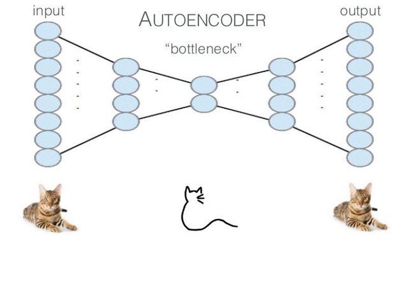
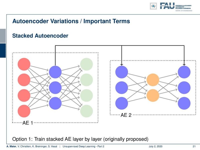
The first image shows a typical layered structure, emphasizing the symmetrical nature often found in autoencoders. The second image illustrates the dimensionality reduction in the encoder and expansion in the decoder, highlighting the bottleneck layer where the compressed representation resides.
Key Hyperparameters for Autoencoders
Choosing the right hyperparameters is crucial for training an effective autoencoder. This table summarizes some key parameters and common choices or considerations.
| Hyperparameter | Description | Common Choices / Considerations |
|---|---|---|
| Encoding Dimension (Bottleneck Size) | The dimensionality of the compressed latent space. | Significantly smaller than input dimension. Depends on data complexity and desired compression level. Too small may lose information; too large may not learn useful compression. Often tuned experimentally. Values like 16, 32, 64, 128 are common starting points. |
| Number of Hidden Layers | Depth of the encoder and decoder. | Deeper networks can potentially learn more complex mappings but risk overfitting. Start simple (1-3 hidden layers per encoder/decoder) and increase complexity if needed. |
| Neurons per Hidden Layer | Width of the hidden layers. | Often follows a funnel shape (decreasing neurons in encoder, increasing in decoder). E.g., Input -> 128 -> 64 -> 32 (bottleneck) -> 64 -> 128 -> Output. |
| Activation Functions (Hidden) | Function applied to hidden layer outputs. | ReLU is a common and effective choice. LeakyReLU, ELU can sometimes help with dying ReLU issues. |
| Activation Function (Output) | Function applied to the final decoder layer. | Depends on input data normalization. 'Sigmoid' if input scaled to [0, 1]. 'Linear' if input is standardized (like StandardScaler output). 'Tanh' if input scaled to [-1, 1]. |
| Optimizer | Algorithm used to update network weights. | 'Adam' is a robust and popular default choice. Adamax, RMSprop are alternatives. Learning rate is a key parameter within the optimizer. |
| Loss Function | Measures the difference between input and reconstruction. | 'mean_squared_error' (MSE) for continuous data. 'binary_crossentropy' if input data is binary (e.g., pixel values scaled 0-1). |
| Epochs | Number of full passes through the training dataset. | Set a relatively high number (e.g., 50, 100, 200) and rely on Early Stopping to find the optimal point. |
| Batch Size | Number of samples processed before the model's internal parameters are updated. | Powers of 2 are common (e.g., 32, 64, 128, 256). Larger batches can speed up training but may generalize slightly worse. Smaller batches introduce more noise but can sometimes help escape local minima. Limited by GPU memory. |
Visual Guide: Building an Autoencoder in Keras
This video provides a practical walkthrough of implementing a basic autoencoder using Keras, covering similar steps to those outlined above, which can be helpful for visual learners.
The tutorial demonstrates setting up the model layers, compiling the autoencoder, and training it on a dataset (often MNIST for image reconstruction examples). Watching how the code translates into network behavior can solidify understanding of the concepts like encoding, decoding, and reconstruction loss.
Frequently Asked Questions (FAQ)
What exactly is the 'bottleneck' in an autoencoder?
The bottleneck is the layer in the autoencoder with the smallest number of neurons, located between the encoder and the decoder. Its purpose is to force the network to learn a compressed representation of the input data. By constraining the information flow through this narrow layer, the encoder must learn to capture the most salient and essential features of the data, discarding noise and redundancy. The dimensionality of this bottleneck layer determines the degree of compression and is a critical hyperparameter.
How do I choose the right encoding dimension (bottleneck size)?
Choosing the optimal encoding dimension is often empirical and depends on the specific dataset and task. There's a trade-off:
- Too small: The network might struggle to capture enough information to reconstruct the input accurately (high reconstruction error), potentially losing important details (underfitting).
- Too large: The network might simply learn an identity function (copying the input) without performing meaningful compression or feature learning. It might overfit the training data.
Start with a reasonable fraction of the input dimension (e.g., 1/4, 1/8) and experiment. Evaluate based on reconstruction loss and, more importantly, the performance of the downstream task (like clustering quality using the Silhouette score or other relevant metrics) using the extracted latent features.
What's the difference between PCA and Autoencoders for dimensionality reduction?
Both PCA (Principal Component Analysis) and Autoencoders can be used for dimensionality reduction, but they differ significantly:
- Linearity: PCA is a linear technique. It finds principal components (linear combinations of original features) that maximize variance. Autoencoders, using non-linear activation functions in their hidden layers, can capture complex non-linear relationships in the data.
- Complexity: PCA is computationally efficient and deterministic (provides the same result every time). Autoencoders require iterative training (like other neural networks), can be computationally more intensive, and results might vary slightly due to random initialization.
- Flexibility: Autoencoders offer more flexibility in architecture design (number of layers, neurons, activation functions) allowing them to potentially model data structures that PCA cannot capture effectively.
In essence, if the underlying structure of your data is primarily linear, PCA is often sufficient and faster. If complex, non-linear patterns are present, an autoencoder might provide a more powerful representation, potentially leading to better results in tasks like clustering.
Can autoencoders be used for anomaly detection?
Yes, autoencoders are commonly used for anomaly detection. The core idea relies on the reconstruction error. An autoencoder is typically trained on 'normal' data (data without anomalies). Since it learns to reconstruct this normal data well, it should exhibit low reconstruction error on similar, unseen normal data points.
However, when presented with an anomaly (a data point significantly different from the training data), the autoencoder will struggle to reconstruct it accurately, resulting in a high reconstruction error. By setting a threshold on the reconstruction error (e.g., based on the distribution of errors on a validation set of normal data), one can flag data points exceeding this threshold as potential anomalies.
References
- Autoencoders: A comprehensive guide to autoencoder architectures - V7 Labs
- What is an Autoencoder? - IBM
- Building Autoencoders in Keras - The Keras Blog
- Autoencoders with Keras, TensorFlow, and Deep Learning - PyImageSearch
- Autoencoder Keras Tutorial - DataCamp
- Autoencoder - Wikipedia
- Introduction to autoencoders - Jeremy Jordan
Recommended
Last updated April 5, 2025