What is Linear Regression?

Understanding the Foundations and Applications of Linear Regression

Key Takeaways

Modeling Relationships: Linear regression effectively models the relationship between dependent and independent variables.
Assumptions Matter: The accuracy of linear regression relies on key statistical assumptions being met.
Wide Applications: From finance to healthcare, linear regression is a versatile tool for prediction and analysis.

Introduction

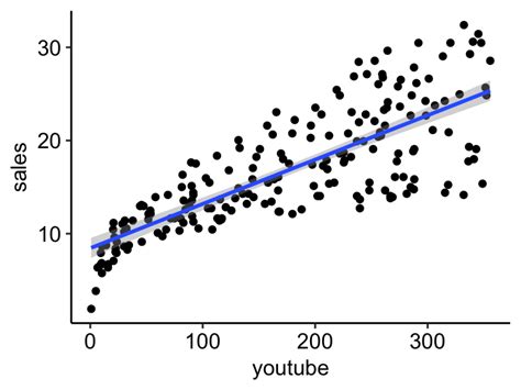
Linear regression is a cornerstone statistical and machine learning technique used to model the relationship between a dependent variable and one or more independent variables. By fitting a linear equation to observed data, it enables predictions and insights into how changes in predictors influence the outcome. Its simplicity and interpretability make it a widely adopted method across various fields.

Key Concepts

Dependent and Independent Variables

In linear regression, the dependent variable (Y) is the outcome or the variable you aim to predict or explain. The independent variable(s) (X) are the predictors or features that influence the dependent variable.

Linear Relationship

The technique assumes a linear relationship between the dependent and independent variables, meaning that changes in the predictors result in proportional changes in the outcome. This relationship is represented by the equation of a straight line in simple linear regression or a hyperplane in multiple linear regression.

Regression Equation

The general form of the linear regression model is:

$$Y = \beta_0 + \beta_1X_1 + \beta_2X_2 + \dots + \beta_nX_n + \epsilon$$

Y: Dependent variable.
β₀: Intercept, representing the value of Y when all X's are zero.
β₁, β₂, ..., βₙ: Coefficients indicating the change in Y for a one-unit change in the respective X.
X₁, X₂, ..., Xₙ: Independent variables.
ε: Error term accounting for variability not explained by the model.

Types of Linear Regression

Simple Linear Regression

Simple linear regression involves only one independent variable. Its equation is:

$$Y = \beta_0 + \beta_1X + \epsilon$$

Here, the relationship between X and Y is depicted as a straight line.

Multiple Linear Regression

Multiple linear regression extends this concept by incorporating two or more independent variables. The equation becomes:

$$Y = \beta_0 + \beta_1X_1 + \beta_2X_2 + \dots + \beta_nX_n + \epsilon$$

This allows for more complex modeling of relationships where multiple factors influence the dependent variable.

Assumptions of Linear Regression

Linearity

The relationship between each independent variable and the dependent variable should be linear. Non-linear relationships can lead to inaccurate models.

Independence

Observations should be independent of each other. This means the value of one observation should not influence another.

Homoscedasticity

The variance of residuals (errors) should be consistent across all levels of the independent variables. Heteroscedasticity, where this variance changes, can undermine the validity of the model.

Normality of Residuals

Residuals should be normally distributed. This assumption is crucial for hypothesis testing and constructing confidence intervals.

No Multicollinearity

Independent variables should not be highly correlated with each other. Multicollinearity can make it difficult to isolate the individual effect of each predictor.

Applications of Linear Regression

Predictive Modeling

Linear regression is extensively used to forecast outcomes such as sales figures, stock prices, or patient health indicators based on historical data.

Trend Analysis

By modeling relationships over time, linear regression helps in identifying and interpreting trends within data sets, aiding in strategic planning and decision-making.

Risk Assessment

In fields like finance and healthcare, linear regression evaluates how different variables impact risk factors, enabling better risk management strategies.

Scientific Research

Researchers use linear regression to understand the relationship between experimental variables, facilitating hypothesis testing and theory development.

Market Research

Market analysts utilize linear regression to determine how factors like advertising spend influence consumer behavior and sales performance.

Advantages of Linear Regression

Simplicity: Straightforward to understand and implement, making it accessible for beginners and professionals alike.
Interpretability: Provides clear coefficients that explain the relationship between each predictor and the outcome.
Computational Efficiency: Requires relatively low computational resources compared to more complex models.
Foundation for Other Models: Acts as a baseline in many machine learning algorithms, aiding in the development of more sophisticated models.

Limitations of Linear Regression

Assumption Dependent: Relies heavily on statistical assumptions which, if violated, can lead to misleading results.
Sensitivity to Outliers: Outliers can disproportionately influence the regression line, skewing the results.
Linear Relationship Requirement: Cannot effectively model complex, non-linear relationships without transformation or extension.
Multicollinearity Issues: High correlation among independent variables can make it difficult to determine individual predictor effects.

How to Perform Linear Regression

Step-by-Step Process

Data Collection: Gather data for the dependent and independent variables relevant to the analysis.
Data Preprocessing:
- Handle missing values through imputation or removal.
- Encode categorical variables if necessary.
- Scale or normalize data to ensure uniformity.
Exploratory Data Analysis (EDA):
- Visualize data distributions and relationships using scatter plots and correlation matrices.
- Identify potential outliers or anomalies.
Model Building:
- Choose the type of linear regression (simple or multiple).
- Fit the model using statistical software or programming languages like Python or R.
- Estimate the coefficients using methods such as Ordinary Least Squares (OLS).
Assumption Validation:
- Check linearity through residual plots.
- Assess homoscedasticity by examining the spread of residuals.
- Evaluate multicollinearity using Variance Inflation Factor (VIF).
- Test for normality of residuals using Q-Q plots or statistical tests like Shapiro-Wilk.
Model Evaluation:
- Use metrics such as R-squared, Adjusted R-squared, Mean Squared Error (MSE), and p-values to assess model performance.
- Interpret the significance and impact of each predictor.
Prediction: Utilize the fitted model to make predictions on new or unseen data.
Model Refinement:
- Address any violation of assumptions through data transformation or by removing outliers.
- Consider adding or removing predictors based on their significance and impact.

Interpretation of Results

Understanding Coefficients

The coefficients (β) in the regression equation represent the expected change in the dependent variable for a one-unit change in the respective independent variable, holding all other variables constant.

Statistical Significance

Assessing the p-values of coefficients helps determine whether the predictors have a statistically significant relationship with the dependent variable. Typically, a p-value below 0.05 indicates significance.

Model Fit

Metrics like R-squared indicate the proportion of variance in the dependent variable explained by the independent variables. Adjusted R-squared adjusts this value based on the number of predictors, providing a more accurate measure when multiple variables are involved.

Example

Predicting House Prices

Consider a scenario where you aim to predict the price of a house based on its size. Using simple linear regression, the relationship can be modeled as:

$$\text{Price} = \beta_0 + \beta_1 \times \text{Size} + \epsilon$$

If the fitted model yields:


# Example: Simple Linear Regression in Python
import numpy as np
import matplotlib.pyplot as plt
from sklearn.linear_model import LinearRegression

# Sample data
size = np.array([1500, 1600, 1700, 1800, 1900]).reshape(-1, 1)
price = np.array([300000, 320000, 340000, 360000, 380000])

# Create and fit the model
model = LinearRegression()
model.fit(size, price)

# Model coefficients
intercept = model.intercept_  # β₀
slope = model.coef_[0]        # β₁

print(f"Intercept (β₀): {intercept}")
print(f"Slope (β₁): {slope}")

# Prediction
predicted_price = model.predict([[2000]])
print(f"Predicted Price for 2000 sqft: {predicted_price[0]}")

# Plotting
plt.scatter(size, price, color='blue')
plt.plot(size, model.predict(size), color='red')
plt.xlabel('Size (sqft)')
plt.ylabel('Price ($)')
plt.title('House Price vs. Size')
plt.show()

Output:

Intercept (β₀): 100000
Slope (β₁): 100
Predicted Price for 2000 sqft: 300000

Interpretation: For every additional square foot, the price of the house increases by $100. A house with 2000 sqft is predicted to cost $300,000.

Advanced Topics

Regularization Techniques

To prevent overfitting, especially in multiple linear regression, regularization methods such as Ridge Regression and Lasso Regression are employed. These techniques add a penalty term to the loss function to constrain the magnitude of the coefficients.

Polynomial Regression

When the relationship between variables is non-linear, polynomial regression extends linear models by incorporating polynomial terms, allowing for curved relationships while maintaining linearity in parameters.

Interactions and Non-Additivity

Incorporating interaction terms between independent variables can model scenarios where the effect of one predictor on the dependent variable depends on the level of another predictor.

Comparative Analysis

Simple vs. Multiple Linear Regression

Aspect	Simple Linear Regression	Multiple Linear Regression
Number of Predictors	One independent variable	Two or more independent variables
Equation Complexity	Y = β₀ + β₁X + ε	Y = β₀ + β₁X₁ + β₂X₂ + ... + βₙXₙ + ε
Visualization	2D scatter plot with a straight line	Higher-dimensional space; visualization is complex
Interpretability	High, easy to interpret slope and intercept	More complex due to multiple coefficients
Use Cases	Simple predictive scenarios with one predictor	Complex scenarios involving multiple factors

Mathematical Foundations

Ordinary Least Squares (OLS)

The most common method for estimating the coefficients in linear regression is Ordinary Least Squares (OLS). OLS minimizes the sum of the squared differences between the observed values and those predicted by the model.

$$\text{Minimize} \sum_{i=1}^{n} (Y_i - (\beta_0 + \beta_1X_{i1} + \dots + \beta_nX_{in}))^2$$

Gradient Descent

For large datasets or more complex models, Gradient Descent can be used to iteratively find the optimal coefficients by minimizing the loss function.

$$\beta_j := \beta_j - \alpha \frac{\partial}{\partial \beta_j} \sum_{i=1}^{n} (Y_i - \hat{Y}_i)^2$$

Practical Implementation

Using Python's Scikit-Learn


from sklearn.linear_model import LinearRegression
from sklearn.model_selection import train_test_split
from sklearn.metrics import mean_squared_error, r2_score
import pandas as pd

# Load dataset
data = pd.read_csv('data.csv')
X = data[['feature1', 'feature2']]
y = data['target']

# Split data
X_train, X_test, y_train, y_test = train_test_split(X, y, test_size=0.2, random_state=42)

# Initialize and train model
model = LinearRegression()
model.fit(X_train, y_train)

# Predictions
y_pred = model.predict(X_test)

# Evaluation
mse = mean_squared_error(y_test, y_pred)
r2 = r2_score(y_test, y_pred)

print(f"MSE: {mse}")
print(f"R-squared: {r2}")

Conclusion

Linear regression remains a fundamental tool in statistical analysis and machine learning due to its simplicity, interpretability, and effectiveness in modeling linear relationships. While it has its limitations, understanding its principles and applications provides a solid foundation for more advanced analytical techniques. Proper adherence to its assumptions and thoughtful model building can yield valuable insights and accurate predictions across a multitude of domains.

References

aws.amazon.com
Last updated January 19, 2025