Linear Shooting Method: Advantages, Disadvantages, Comparison, and Real-Life Applications

A comprehensive analysis of the linear shooting approach for boundary value problems

Key Takeaways

Efficiency in Simplicity: The method transforms boundary value problems into initial value problems, leveraging existing IVP solvers for simplicity and speed in linear contexts.
Sensitivity and Limitations: Its reliance on precise initial guesses means that instability and divergence may occur, especially in problems with growing modes or when extending to nonlinear cases.
Methodological Trade-Offs: While it is intuitive and computationally efficient for many 1D linear problems, alternative approaches like finite difference, finite element, and collocation methods offer more robustness for complex or non-linear problems.

Introduction

The linear shooting method is a well-established numerical technique used primarily for solving two-point boundary value problems (BVPs) in ordinary differential equations (ODEs). This approach involves converting a BVP into one or more initial value problems (IVPs). By “shooting” from one end of the domain and adjusting the unknown initial conditions iteratively, the method seeks a solution that meets the boundary conditions at the other end. Its simplicity and the ability to leverage mature IVP solving techniques make it a popular choice in many scientific and engineering applications.

While naturally suited to linear differential systems, the linear shooting method’s extension to more complicated systems, particularly nonlinear problems, introduces additional challenges. Despite these challenges, its practical efficacy in numerous fields such as heat transfer, quantum mechanics, fluid dynamics, and structural analysis has ensured its enduring relevance.

Understanding the Linear Shooting Method

Fundamental Concept

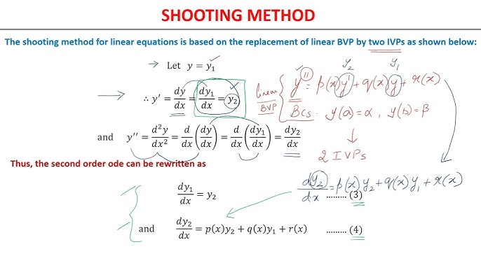
At its core, the linear shooting method involves converting a BVP into an IVP. In a typical boundary value problem, conditions are specified at two separate points on the domain (for example, at the endpoints of an interval). The shooting method begins by assuming an initial guess for the unknown initial condition(s) at the starting point. The ODE is then integrated using a standard IVP solver (such as the Runge–Kutta method), and the solution is evaluated at the end boundary.

If the solution meets the boundary condition at the other end, the selected initial guess is considered correct. If not, the guess is adjusted iteratively—often using linear interpolation or by setting up an algebraic relation based on the superposition principle (a beneficial property in linear systems)—until convergence is achieved.

Mathematical Formulation

Consider a second-order linear differential equation where the boundary conditions are given as:

$$ y''(x) = F(x, y, y'), \quad y(a) = \alpha, \quad y(b) = \beta. $$ The shooting method starts by guessing a value for the derivative at the initial point, say, $y'(a)=s$. The resulting initial value problem is solved over the interval $[a, b]$, and the computed $y(b)$ is compared with $\beta$. The process is repeated iteratively using the linearity of the problem to adjust the guess $s$ until $y(b)$ sufficiently approximates $\beta$.

Advantages of the Linear Shooting Method

1. Simplicity and Ease of Implementation

The linear shooting method is straightforward to both understand and implement. Given that it converts a BVP into one or more IVPs, it can utilize well-established solvers that have been refined over decades. This advantage is crucial for practitioners who require an intuitive and less complex numerical method.

In linear systems, where the superposition principle applies, the adjustment of initial guesses can even be managed analytically in some cases. The fundamental procedure—setting up initial conditions, integrating over the domain, and adjusting the guesses—remains both conceptually simple and practically efficient.

2. Efficiency in Low-Dimensional Problems

For many low-dimensional boundary value problems, the shooting method is highly efficient. When the system of ODEs does not exhibit excessive stiffness and the dimension is manageable, the iterative process converges quickly. This efficiency is enhanced by the availability of adaptive IVP solvers which provide accurate solutions with minimal computational overhead.

3. Utilization of Robust IVP Solvers

One of the method's defining strengths is its compatibility with efficient and adaptive IVP solvers. These solvers, such as variants of the Runge-Kutta methods, have been profoundly optimized over the years, offering high accuracy and reliability. By leveraging these solvers, the shooting method can achieve high precision, particularly for linear systems where the relationship between initial conditions and the boundary conditions is more predictive.

Disadvantages of the Linear Shooting Method

1. Sensitivity to Initial Guesses

The accuracy of the linear shooting method is heavily dependent on the quality of the initial guess for the unknown initial condition. A poor choice can lead to significant divergence from the desired boundary value, or it might require many iterations to converge. In systems characterized by strong sensitivity or where there are rapidly growing modes, even slight deviations in the guess can multiply, leading to unstable or divergent solutions.

2. Instability in Stiff Problems

In cases where the differential equation exhibits stiffness, the sensitivity to initial conditions becomes even more problematic. Small errors in the guess can result in exponential growth (or decay) of errors during integration, making it challenging to satisfy the endpoint conditions. This instability often limits the method's applicability to less stiff or moderately stiff problems.

3. Limitations for Nonlinear Problems

Although the linear shooting method is primarily designed for linear problems, its extension to nonlinear differential equations is fraught with additional complexities. Nonlinear systems often do not benefit from the superposition principle, and the iterative process becomes more intensive, requiring sophisticated methods for guessing and adjusting initial conditions. As a result, alternative approaches such as Newton’s method combined with shooting may be necessary, thereby diminishing the method’s intrinsic simplicity.

4. Limited Robustness for Complex Geometries

When boundary conditions are defined in complex geometries or involve higher-order derivatives, the straightforward approach of the shooting method may fail to provide robust or unique solutions. The method can become cumbersome when extended beyond one-dimensional domains or simple boundary conditions, making other numerical techniques more attractive in such scenarios.

Comparison with Other Numerical Models

Overview

Several alternative numerical methods exist for solving boundary value problems, each with its unique strengths and weaknesses. The finite difference method, finite element method, and collocation method are prominent examples. A comparative understanding of these methodologies can aid in selecting the most appropriate approach for a given problem.

Comparison Table

Method	Advantages	Disadvantages
Shooting Method	Simple implementation for one-dimensional linear BVPs Utilizes robust IVP solvers Conceptually intuitive	Sensitive to initial guesses Instability in stiff or rapidly varying problems Less effective for nonlinear or complex geometries
Finite Difference Method (FDM)	Robust and stable for a wide array of problems Direct discretization offers a global solution overview	May require significant memory and computational resources Less intuitive due to complex discretization schemes
Finite Element Method (FEM)	Highly flexible for complex geometries and non-linear problems Suitable for multi-dimensional domains	More complex implementation and higher computational cost Requires specialized knowledge in meshing and function approximation
Collocation Methods	High accuracy for smooth problems using global approximations Efficient for problems with rapid changes if nodes are chosen appropriately	Requires careful selection of basis functions and nodes Implementation can be more involved for non-standard boundary conditions

This table highlights the trade-offs between the shooting method and its alternatives. While the shooting method stands out for its simplicity and the effective use of existing IVP solvers, alternative methods such as finite difference and finite element approaches offer greater stability and flexibility, especially for problems with higher dimensionality or nonlinearity.

Real-Life Applications

Engineering Applications

In structural analysis, the shooting method is applied to determine the deflection and stress distribution in beams and columns under various loading conditions. For instance, when analyzing a beam with fixed-end supports and variable cross-sectional properties, the method can be used to solve the corresponding ODEs to predict bending behavior and ensure that the structural design meets safety requirements.

Similarly, in aerospace engineering, trajectory computations for projectiles and spacecraft benefit from the shooting method. By iterating on initial launch conditions, engineers can determine the precise paths needed to ensure that vehicles meet their targeted endpoints, accounting for gravitational influences and atmospheric drag.

Heat Transfer and Diffusion Problems

The shooting method is notably employed in solving problems involving heat transfer and diffusion. For example, in the design of heat exchangers, it is crucial to predict the temperature distribution along the length of a material. By formulating the temperature profile as a boundary value problem with defined temperatures at both ends of a medium, the shooting method provides an efficient route to model the thermal gradients.

In chemical engineering, the analysis of concentration profiles in reactors is essential. Chemical reactions often involve diffusion processes where the concentrations of reactants and products are fixed at the boundaries. The shooting method aids in resolving the differential equations governing these profiles, thereby ensuring optimal reactor design and operation.

Quantum Mechanics

One of the most prominent applications of the linear shooting method is found in quantum mechanics. When solving the Schrödinger equation for one-dimensional potential wells, the shooting method helps determine the energy eigenvalues and corresponding wavefunctions. By adjusting the initial conditions iteratively until the boundary conditions of the quantum system are satisfied, the method allows physicists to predict energy levels with high accuracy. This application not only exemplifies the method’s precision in linear domains but also its utility in fundamental research.

Fluid Dynamics and Boundary Layer Analysis

In fluid dynamics, especially in the study of laminar boundary layers, the shooting method is used to solve the Blasius equation—a classical BVP that models the velocity profile of a fluid near a solid surface. The method’s ability to manage the integration from the wall to the free stream, adjusting the initial guesses iteratively, makes it an invaluable tool for analyzing flow characteristics, which is vital for optimizing aerodynamic designs.

Environmental and Economic Modeling

Beyond traditional engineering disciplines, the linear shooting method finds applications in environmental and economic models where boundary conditions may represent fixed concentrations or cost constraints. For example, in modeling pollutant diffusion in soil or analyzing spatial economic distributions, the method can be employed to understand how variables change over a region, providing important insights for policymakers and researchers alike.

Conclusion

In conclusion, the linear shooting method remains a cornerstone numerical technique for tackling boundary value problems, particularly within the realm of linear ordinary differential equations. Its primary strengths lie in its simplicity, efficiency, and the ability to harness well-established IVP solvers. However, the method does have its limitations—notably, its sensitivity to initial guesses and instability in stiff or complex scenarios. Whilst alternative methods such as finite difference, finite element, and collocation methods offer enhanced robustness and flexibility, the shooting method continues to deliver outstanding performance for a variety of applications including structural analysis, thermal modeling, quantum mechanics, and fluid dynamics. The choice of method ultimately depends on the problem’s specific characteristics, including the dimensionality, nonlinearity, and the complexity of the boundary conditions.