
Understanding and Optimizing Large Language Model Inference
A Comprehensive Guide with Code Examples and Best Practices
Key Takeaways
- Comprehensive Inference Pipeline: Grasp the full process from tokenization to output generation in LLMs.
- Transformer and Mixture of Experts: Understand the core components and specialized architectures that enhance model performance.
- Optimization Techniques: Learn effective strategies to reduce latency and computational costs without compromising quality.
1. Introduction to Large Language Model Inference
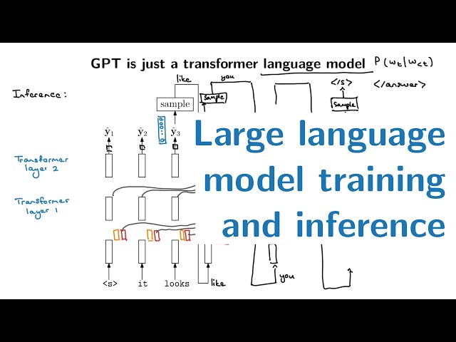
Large Language Models (LLMs) such as GPT-4 have revolutionized natural language processing by enabling machines to generate human-like text. Understanding the inference process of these models is crucial for deploying them effectively in various applications. This guide delves into the detailed steps involved in LLM inference, including tokenization, transformer operations, Mixture of Experts (MoE) architectures, and optimization techniques aimed at reducing latency and cost.
2. Tokenization: Converting Words to Tokens
2.1. What is Tokenization?
Tokenization is the foundational step in LLM inference, where raw text is transformed into numerical representations that models can process. This involves breaking down text into smaller units called tokens, which can represent words, subwords, or even individual characters.
2.2. Tokenization Methods
2.2.1. Byte-Pair Encoding (BPE)
BPE is a subword tokenization technique that iteratively merges the most frequent pair of bytes or characters in a dataset. This method efficiently handles rare and compound words by breaking them into more frequent subword units.
2.2.2. WordPiece
Similar to BPE, WordPiece tokenization focuses on maintaining the integrity of the language model's prediction targets by optimizing the subword units based on frequency and context.
2.2.3. SentencePiece
SentencePiece treats the input text as a raw byte sequence, enabling it to handle languages without explicit word boundaries and supporting various tokenization schemes like BPE and Unigram.
2.3. Tokenization Process
The tokenization process typically involves the following steps:
- Text Preprocessing: Cleans and normalizes the input text by removing unnecessary symbols, punctuation, or applying lowercasing if needed.
- Token Splitting: Divides the text into tokens using algorithms like BPE or WordPiece.
- Mapping to IDs: Each token is mapped to a unique integer ID based on the model's vocabulary.
- Padding and Truncation: Adjusts the sequence length to a fixed size by adding padding tokens or truncating excess tokens.
2.4. Python Example: Tokenization with Hugging Face
from transformers import AutoTokenizer

# Initialize tokenizer
tokenizer = AutoTokenizer.from_pretrained("gpt2")

# Input text
input_text = "How does inference work in large language models?"

# Tokenize the text
tokens = tokenizer.encode_plus(
    input_text,
    max_length=512,
    padding="max_length",
    truncation=True,
    return_tensors="pt"  # PyTorch format tensor
)

print("Input IDs:", tokens["input_ids"])
print("Attention Mask:", tokens["attention_mask"])
Explanation: This code snippet demonstrates how to use the Hugging Face Transformers library to tokenize input text. The tokenizer converts the text into token IDs and generates an attention mask to indicate valid tokens versus padding.
3. Transformer Architecture in LLM Inference
3.1. Overview of Transformer Layers
The transformer architecture is the backbone of modern LLMs, enabling them to capture complex dependencies in data through self-attention mechanisms and feed-forward networks. Each transformer layer typically consists of the following components:
3.1.1. Embedding and Positional Encoding
Tokens are first converted into dense vector embeddings. Since transformers lack inherent sequential processing, positional encoding is added to these embeddings to retain information about the order of tokens.
3.1.2. Self-Attention Mechanism
The self-attention mechanism allows each token to attend to other tokens in the sequence, capturing contextual relationships. It operates by computing query (Q), key (K), and value (V) matrices for each token and calculating attention scores.
3.1.3. Feed-Forward Networks (FFN)
After self-attention, each token's representation is passed through a feed-forward network, typically consisting of two linear layers with a non-linear activation function like GeLU in between.
3.1.4. Layer Normalization and Residual Connections
Layer normalization stabilizes the training process, while residual connections help in mitigating the vanishing gradient problem, allowing the model to learn deeper representations.
3.2. Self-Attention Detailed
Self-attention computes how much focus each token should have on every other token in the sequence. The attention mechanism is defined mathematically as:
$$Attention(Q, K, V) = Softmax\left(\frac{Q \cdot K^\top}{\sqrt{d_k}}\right) \cdot V$$
Where:
-
Q: Query matrix derived from the input embeddings.
-
K: Key matrix derived from the input embeddings.
-
V: Value matrix derived from the input embeddings.
-
d_k: Dimension of the key vectors, used for scaling.
3.3. Stacking Transformer Layers
Multiple transformer layers are stacked on top of each other to deepen the model, enhancing its capacity to capture intricate patterns and dependencies within the data.
3.4. Python Example: Transformer Layer Implementation
import torch
import torch.nn as nn

class TransformerLayer(nn.Module):
    def __init__(self, embed_dim, num_heads, dropout=0.1):
        super().__init__()
        self.self_attn = nn.MultiheadAttention(embed_dim, num_heads, dropout=dropout)
        self.feed_forward = nn.Sequential(
            nn.Linear(embed_dim, embed_dim * 4),
            nn.GELU(),
            nn.Linear(embed_dim * 4, embed_dim)
        )
        self.layer_norm1 = nn.LayerNorm(embed_dim)
        self.layer_norm2 = nn.LayerNorm(embed_dim)
        self.dropout = nn.Dropout(dropout)

    def forward(self, x, src_mask=None, src_key_padding_mask=None):
        # Self-attention
        attn_output, _ = self.self_attn(x, x, x, attn_mask=src_mask, key_padding_mask=src_key_padding_mask)
        x = x + self.dropout(attn_output)
        x = self.layer_norm1(x)

        # Feed-forward network
        ff_output = self.feed_forward(x)
        x = x + self.dropout(ff_output)
        x = self.layer_norm2(x)

        return x

# Example usage
embed_dim = 512
num_heads = 8
transformer_layer = TransformerLayer(embed_dim, num_heads)

# Dummy input: (sequence_length, batch_size, embed_dim)
x = torch.randn(10, 32, embed_dim)
output = transformer_layer(x)
print("Output shape:", output.shape)
Explanation: This code defines a transformer layer with self-attention, a feed-forward network, layer normalization, and dropout for regularization. It processes a dummy input tensor and outputs the transformed representation.
4. Mixture of Experts (MoE) in LLM Inference
4.1. Introduction to Mixture of Experts
Mixture of Experts (MoE) is an architectural innovation designed to scale LLMs efficiently. It involves multiple expert networks and a gating mechanism that dynamically selects relevant experts for each input, thereby enhancing scalability without proportionally increasing computational costs.
4.2. Components of MoE
4.2.1. Experts
Experts are specialized sub-models, typically feed-forward neural networks, that handle different aspects of the input. Each expert is trained to focus on specific patterns or features within the data.
4.2.2. Gating Network
The gating network assigns input tokens to specific experts based on learned routing weights. It ensures that only a subset of experts is activated for any given input, thereby reducing computational overhead.
4.2.3. Aggregation Mechanism
After processing, the outputs from the selected experts are aggregated, typically by weighting them according to the gating scores. This combined output represents the final transformation for the input tokens.
4.3. Advantages of MoE
- Scalability: Allows the model to scale to trillion-parameter sizes without a linear increase in computation.
- Efficiency: Activates only a subset of experts, reducing the computational load per inference.
- Diversity: Enables specialization of experts, enhancing the model's ability to handle diverse tasks.
4.4. Python Example: Simplified MoE Implementation
import torch
import torch.nn as nn
import torch.nn.functional as F

class MixtureOfExperts(nn.Module):
    def __init__(self, embed_dim, num_experts, expert_dim=1024):
        super().__init__()
        self.num_experts = num_experts
        self.router = nn.Linear(embed_dim, num_experts)
        self.experts = nn.ModuleList([nn.Sequential(
            nn.Linear(embed_dim, expert_dim),
            nn.ReLU(),
            nn.Linear(expert_dim, embed_dim)
        ) for _ in range(num_experts)])

    def forward(self, x):
        # Compute routing weights
        routing_weights = F.softmax(self.router(x), dim=-1)  # Shape: (batch_size, seq_length, num_experts)

        # Initialize output tensor
        output = torch.zeros_like(x)

        # Distribute tokens to experts
        for expert_idx in range(self.num_experts):
            # Select tokens routed to the current expert
            expert_mask = routing_weights[:, :, expert_idx].unsqueeze(-1)  # Shape: (batch_size, seq_length, 1)
            expert_input = x * expert_mask  # Masked input for the expert

            # Process through the expert
            expert_output = self.experts[expert_idx](expert_input)

            # Aggregate the expert's output
            output += expert_output * expert_mask

        return output

# Example usage
embed_dim = 512
num_experts = 4
moe = MixtureOfExperts(embed_dim, num_experts)

# Dummy input: (batch_size, seq_length, embed_dim)
x = torch.randn(32, 10, embed_dim)
output = moe(x)
print("Output shape:", output.shape)
Explanation: This simplified MoE class routes each token to multiple experts using a gating mechanism. The router computes softmax weights for each expert, and the input is selectively processed by the activated experts. The outputs are then aggregated based on the routing weights.
5. Optimization Techniques for Reducing Latency and Cost
5.1. Model Compression
5.1.1. Pruning
Pruning involves removing redundant or less significant weights and connections from the model, thereby reducing its size and computational requirements without substantially affecting performance.
5.1.2. Quantization
Quantization reduces the numerical precision of model weights from 32-bit floating-point to lower bit representations like 16-bit or 8-bit integers. This decreases memory usage and accelerates computations.
5.1.3. Knowledge Distillation
Knowledge distillation transfers knowledge from a large "teacher" model to a smaller "student" model. The student model learns to mimic the teacher's behavior, achieving similar performance with reduced complexity.
5.2. Inference Optimizations
5.2.1. Caching Past Key/Value States
During autoregressive generation, caching the key and value projections from previous tokens avoids redundant computations, significantly speeding up the inference process.
5.2.2. Efficient Attention Mechanisms
Techniques like sparse attention or low-rank approximations reduce the quadratic complexity of the attention mechanism, making it more scalable for longer sequences.
5.2.3. Model and Pipeline Parallelism
Distributing the model across multiple GPUs or nodes allows parallel processing of different parts of the model, enhancing throughput and reducing inference time.
5.2.4. Hardware Acceleration and Specialized Libraries
Leveraging specialized hardware like GPUs, TPUs, or inference-optimized libraries (e.g., NVIDIA TensorRT, ONNX Runtime) can drastically improve inference speed and efficiency.
5.3. Batch Inference
Processing multiple inputs simultaneously in batches can optimize computational resources and reduce per-token latency, especially when deployed on parallel processing architectures.
5.4. Python Example: Quantization with PyTorch
import torch
import torch.nn as nn
from torch.quantization import quantize_dynamic

# Define a simple model
class SimpleModel(nn.Module):
    def __init__(self):
        super().__init__()
        self.fc1 = nn.Linear(512, 1024)
        self.relu = nn.ReLU()
        self.fc2 = nn.Linear(1024, 512)

    def forward(self, x):
        x = self.fc1(x)
        x = self.relu(x)
        x = self.fc2(x)
        return x

# Initialize the model and dummy input
model = SimpleModel()
x = torch.randn(1, 512)

# Quantize the model dynamically
quantized_model = quantize_dynamic(
    model,
    {nn.Linear},  # Layers to quantize
    dtype=torch.qint8  # Quantization data type
)

# Perform inference with the quantized model
output = quantized_model(x)
print("Quantized Output:", output)
Explanation: This example demonstrates dynamic quantization of a simple neural network using PyTorch. The `quantize_dynamic` function converts specified layers (e.g., `nn.Linear`) to lower precision, reducing model size and speeding up inference.
5.5. Optimization Summary Table
| Optimization Technique | Description | Benefits |
|---|---|---|
| Pruning | Removing redundant weights and connections. | Reduces model size and computational load. |
| Quantization | Lowering numerical precision of weights. | Decreases memory usage and speeds up computations. |
| Knowledge Distillation | Training a smaller model to mimic a larger model. | Maintains performance with reduced complexity. |
| Caching Past States | Storing previous key/value pairs in attention. | Avoids redundant computations, speeding up inference. |
| Efficient Attention | Implementing sparse or approximate attention mechanisms. | Reduces computational complexity for longer sequences. |
| Parallelism | Distributing model processing across multiple hardware units. | Enhances throughput and reduces latency. |
| Hardware Acceleration | Utilizing GPUs, TPUs, or specialized libraries. | Improves inference speed and efficiency. |
| Batch Inference | Processing multiple inputs in parallel batches. | Optimizes resource utilization and reduces per-token latency. |
6. References
7. Conclusion
The inference process of large language models encompasses intricate steps from tokenizing input text to generating coherent and contextually relevant outputs. By leveraging transformer architectures and innovations like Mixture of Experts, these models achieve remarkable performance. However, the computational demands necessitate effective optimization strategies to ensure scalability and efficiency. Techniques such as pruning, quantization, caching, and hardware acceleration play pivotal roles in reducing latency and operational costs. Understanding and implementing these components and optimizations are essential for deploying LLMs effectively in real-world applications.
Last updated February 1, 2025