Can Machine Learning Truly Revolutionize Finite Element Meshing? Unpacking the Mathematical Proof

Finite Element Analysis (FEA) is a cornerstone of modern engineering simulation, allowing us to predict how designs behave under real-world conditions. At its heart lies the mesh – a discretization of the physical domain into smaller, simpler elements. The quality and density of this mesh are paramount; too coarse, and the simulation lacks accuracy; too fine, and the computational cost becomes prohibitive. Finding the sweet spot is crucial.

You've hit upon a cutting-edge concept: leveraging Machine Learning (ML) to automate and optimize this mesh generation process. The idea is compelling – an ML system could learn from simulation results, identifying regions prone to high errors or complex phenomena, and dynamically refine the mesh precisely where needed. This promises an intelligent balance between accuracy and computational expense. But the critical question remains: can we mathematically prove that this ML-integrated approach is rigorously better than established, non-ML methods for adaptive mesh refinement (AMR)?

Key Insights: Proving ML's Edge in FEA Meshing

Error Reduction Frameworks: Mathematical proof often involves showing that ML-guided refinement strategies lead to demonstrably lower error bounds (e.g., in energy or L2 norms) compared to traditional heuristic or uniform refinement approaches for a given computational budget.
Optimized Computational Efficiency: Rigorous analysis aims to prove that ML techniques can achieve a target simulation accuracy with significantly fewer mesh elements or degrees of freedom, thus reducing computational time and memory requirements compared to baseline methods.
Data-Driven Policy Optimization: Techniques like Reinforcement Learning (RL) frame mesh adaptation as a sequential decision problem, allowing for proofs based on the convergence of learned policies towards strategies that optimally balance error minimization and computational cost, surpassing fixed heuristics.

Setting the Stage: Traditional Adaptive Mesh Refinement (AMR)

Before diving into ML's role, it's essential to understand conventional AMR techniques. These methods have been the workhorse for decades, improving simulation accuracy by selectively refining the mesh based on indicators of error.

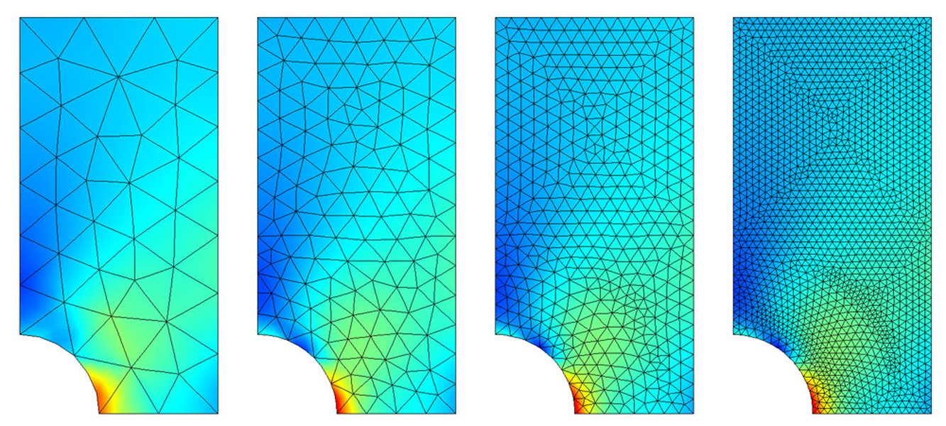
Example of mesh refinement around a stress concentration

Traditional adaptive mesh refinement focuses density around areas of high stress or error gradients.

Error Estimation: The Guiding Principle

Traditional AMR typically relies on a posteriori error estimators. These mathematical tools analyze a completed simulation run on a given mesh to estimate the distribution and magnitude of errors. Common types include:

Residual-Based Estimators: Evaluate how well the approximate solution satisfies the governing partial differential equations (PDEs) within each element and on element boundaries.
Recovery-Based Estimators: Compare the computed solution's gradient (e.g., stress) with a smoother, recovered gradient field. Larger discrepancies suggest higher errors.

These estimators provide quantitative metrics used to decide where the mesh needs more elements.

Refinement Strategies: Heuristics and Rules

Based on the error estimation, refinement strategies are applied. These often involve heuristics, such as:

Refining all elements where the estimated error exceeds a certain threshold.
Refining a fixed percentage of elements with the highest estimated errors.
Employing h-refinement (dividing elements), p-refinement (increasing polynomial order), or r-refinement (moving node locations).

While effective, these methods can sometimes lead to overly conservative refinement or rely heavily on user expertise and problem-specific tuning. They might struggle to find the truly optimal mesh distribution, especially for complex, transient problems where error features evolve dynamically.

Mesh overlaid on a stress plot, showing refinement

Visualizing mesh density correlated with simulation results (e.g., stress).

Enter Machine Learning: A New Paradigm for AMR

ML introduces a fundamentally different approach. Instead of relying solely on pre-defined estimators and heuristics, ML models can *learn* optimal refinement strategies from data, potentially capturing complex relationships between geometry, physics, simulation state, and error patterns that traditional methods might miss.

Diverse ML Approaches

Several ML techniques are being explored for mesh generation and AMR:

Predicting Optimal Densities: Supervised learning models, like Convolutional Neural Networks (CNNs), can be trained on datasets of geometries and their corresponding 'optimal' meshes (generated via expensive methods or expert knowledge) to predict ideal mesh density functions for new problems.
Reinforcement Learning (RL) for Adaptive Control: AMR can be framed as a sequential decision-making problem, solvable with RL. An 'agent' learns a policy (a strategy) to refine or coarsen parts of the mesh at different stages of the simulation. The goal is typically to maximize a reward function that balances accuracy improvement against computational cost. This can be formulated using Markov Decision Processes (MDPs) or even Multi-Agent RL (MARL) where different agents control different mesh regions.
Direct Prediction of Refinement Regions: Deep Learning models (e.g., architectures like ADARNet) can take low-resolution simulation data as input and directly predict which specific regions require higher resolution, effectively learning the error indicators implicitly.
Physics-Informed ML: ML models can be specifically trained to identify and refine regions critical to certain physical phenomena, such as boundary layers, shock waves, or turbulent eddies in fluid dynamics simulations.

The overarching goal is to automate the process, reduce reliance on manual tuning, and achieve superior performance by dynamically tailoring the mesh to the unique features of each simulation.

Constructing the Mathematical Proof: Demonstrating ML's Superiority

Proving mathematically that ML-enhanced AMR is superior requires a rigorous framework comparing it against traditional methods based on well-defined metrics and theoretical principles.

Step 1: Define Clear Metrics and Objectives

Any rigorous comparison needs unambiguous metrics. Key metrics include:

Error Metric \(E\): Quantifies the simulation error. Common choices are norms of the difference between the true solution \(u\) and the finite element approximation \(u_h\), such as the energy norm \( \| u - u_h \|_E \) or the \( L^2 \) norm \( \| u - u_h \|_{L^2} \). Since the true solution \(u\) is usually unknown, reliable *a posteriori* error estimates \( \eta(u_h) \) are often used as a proxy.
Computational Cost \(C\): Measures the resources used. Typically represented by the number of elements (N) or degrees of freedom (DoFs) in the mesh, which correlate strongly with computation time and memory usage.

The objective is usually framed as an optimization problem: \[ \min E \quad \text{subject to} \quad C \leq C_{budget} \] or \[ \min C \quad \text{subject to} \quad E \leq E_{tolerance} \] We need to prove that ML strategies achieve a better trade-off between \(E\) and \(C\).

Step 2: Establish the Baseline Performance

We need the theoretical performance bounds of traditional methods as a reference. For many elliptic PDEs and standard adaptive strategies based on reliable error estimators, theory predicts convergence rates like:

\[ E(N) \leq K_1 N^{-\alpha} \]

where \(N\) is the number of elements/DoFs, \(K_1\) is a constant depending on the problem, and \(\alpha\) is the convergence rate. Optimal adaptive methods aim to achieve the best possible \(\alpha\) for the given problem regularity, even in the presence of singularities.

Step 3: Model the ML Refinement Strategy Mathematically

The ML approach needs a mathematical representation.

For predictive models, this could be a learned function \( f_{ML}: \text{Geometry/State} \to \text{Mesh Density Field} \).

For RL, it's a learned policy \( \pi_{ML}: \text{State} \to \text{Action (Refine/Coarsen)} \), aiming to optimize an expected reward that balances error \(E\) and cost \(C\), often formulated as: \[ \max_{\pi} \mathbb{E} \left[ \sum_{t=0}^T \gamma^t R_t(\pi) \right], \quad \text{where } R_t \approx - (\lambda_E E_t + \lambda_C C_t) \] Here, \(R_t\) is the reward at step \(t\), \(\gamma\) is a discount factor, and \(\lambda_E, \lambda_C\) are weighting factors for error and cost.

Step 4: Prove Improved Error Bounds, Convergence, or Optimality

This is the core of the proof. It involves showing that the ML strategy leads to better outcomes:

Improved Error Bounds: Demonstrate that for a given number of elements \(N\), the error achieved by the ML-generated mesh \(E_{ML}(N)\) is lower than that of the traditional method \(E_{Trad}(N)\), i.e., \( E_{ML}(N) < E_{Trad}(N) \), or that it achieves a better convergence rate constant (\(K_{ML} < K_{Trad}\)).
Faster Convergence Rate: Prove that the ML strategy achieves a higher convergence rate \(\alpha_{ML} > \alpha_{Trad}\), meaning the error decreases more rapidly as elements are added.
Meeting Optimality Conditions: Show that the mesh generated by ML better satisfies theoretical conditions for optimality (e.g., equidistribution of error indicators across elements), which traditional heuristics might only approximate.
Efficiency: Prove that for a target error tolerance \(E_{tolerance}\), the ML approach requires fewer elements/DoFs \(N_{ML} < N_{Trad}\).

This often involves leveraging the theory of *a posteriori* error estimation, showing that the ML policy leads to smaller estimated errors or satisfies reliability and efficiency bounds more effectively.

Step 5: Leverage Learning Theory

Since ML models learn from data, proofs can incorporate concepts from:

Statistical Learning Theory: Provide generalization bounds showing that the ML model's learned refinement strategy performs well not just on training data but on new, unseen simulation scenarios, converging to a near-optimal strategy as more data becomes available.
Reinforcement Learning Theory: Use convergence proofs for RL algorithms (like Q-learning or policy gradients) to show that the learned policy \(\pi_{ML}\) converges towards an optimal policy \(\pi^*\) for the defined MDP, thereby guaranteeing improved performance in terms of expected reward (balancing error and cost).

Visualizing the Comparison: Traditional vs. ML-Enhanced AMR

This radar chart provides a conceptual comparison between traditional AMR techniques and ML-enhanced approaches across several key dimensions. The scores are qualitative, representing potential advantages often cited in research.

This visualization suggests ML approaches have higher potential for accuracy, efficiency, automation, and handling complexity, but may require more initial setup (data collection, model training) and currently have less reliance on well-established heuristics (which can be good or bad depending on context).

Mapping the Proof Structure

The following mindmap outlines the key components involved in mathematically demonstrating the superiority of ML-enhanced Adaptive Mesh Refinement in Finite Element Analysis.

mindmap root["Proof Framework for ML-Enhanced AMR Superiority"] id1["1. Define Metrics & Objectives"] id1a["Error Metrics (E)
e.g., Energy Norm, L2 Norm,
A Posteriori Estimates"] id1b["Computational Cost (C)
e.g., DoFs, Element Count, Time"] id1c["Optimization Goal
Min E for fixed C, or Min C for fixed E"] id2["2. Establish Baseline"] id2a["Traditional AMR Methods
Heuristics, Error Estimators"] id2b["Theoretical Convergence Rates
E(N) <= K * N^-alpha"] id2c["Known Limitations"] id3["3. Model ML Strategy"] id3a["Predictive Models (e.g., CNN)
Mapping Geometry -> Mesh Density"] id3b["Reinforcement Learning (RL)
Policy pi: State -> Action
Reward Function (Error vs Cost)"] id3c["Direct Prediction (e.g., DL)"] id4["4. Core Proof Techniques"] id4a["Improved Error Bounds
E_ML < E_Trad for same C"] id4b["Faster Convergence Rates
alpha_ML > alpha_Trad"] id4c["Enhanced Efficiency
N_ML < N_Trad for same E"] id4d["Satisfying Optimality Conditions
e.g., Error Equidistribution"] id5["5. Leverage Theoretical Frameworks"] id5a["A Posteriori Error Estimation Theory
Reliability & Efficiency"] id5b["Statistical Learning Theory
Generalization Bounds"] id5c["Reinforcement Learning Theory
Policy Convergence, Performance Guarantees"] id6["6. Validation"] id6a["Numerical Experiments
Benchmarking on Test Cases"] id6b["Analysis on Simplified Problems"]

This map illustrates the multi-faceted nature of the proof, requiring elements from numerical analysis, optimization theory, and machine learning theory.

Comparing Approaches: Traditional vs. ML-Enhanced AMR

The table below summarizes key characteristics and differences between traditional and ML-enhanced adaptive mesh refinement approaches based on the synthesis of current research.

Feature	Traditional AMR	ML-Enhanced AMR
Driving Mechanism	A posteriori error estimators (e.g., residual, recovery-based) + Heuristics	Learned models (Predictive, RL policies) trained on simulation data/errors
Adaptation Strategy	Often rule-based (e.g., refine elements above error threshold)	Data-driven, potentially capturing complex error patterns; policy optimizes error/cost balance
Automation	Semi-automated, often requires parameter tuning and expert input	Higher potential for full automation once trained
Optimality	Aims for optimality via established theory, but heuristics may be suboptimal	Can potentially learn near-optimal strategies directly from data, especially via RL
Handling Complexity	Can struggle with highly complex geometries or rapidly changing transient phenomena	Potentially better suited for complex/dynamic problems by learning underlying patterns
Development Cost	Relatively well-understood algorithms, lower initial barrier	Requires data generation, ML model training, potentially higher initial development effort
Theoretical Foundation	Strong foundation in numerical analysis and PDE theory	Combines numerical analysis with learning theory (statistical learning, RL theory)
Generalizability	Established methods generally applicable, but tuning might be needed	Model generalizability depends on training data diversity; potential need for retraining

Exploring Adaptive Mesh Optimization

The following video from Lawrence Livermore National Laboratory discusses R-Adaptive Mesh Optimization, a technique related to improving mesh quality by moving nodes (r-adaptation), which complements h-adaptation (refinement/coarsening) often targeted by ML.

This video delves into optimization techniques used to enhance mesh quality for finite element methods, highlighting the mathematical complexities and goals involved in ensuring simulation accuracy and robustness, concepts central to proving the effectiveness of any mesh improvement strategy, including ML-based ones.

The Practical Reality: Proof vs. Performance

While the pathway to mathematical rigor exists, achieving a universal, mathematically airtight proof that ML *always* outperforms traditional AMR for *any* PDE, geometry, and ML model is extremely challenging, perhaps impossible due to principles like the "No Free Lunch" theorems in optimization. These theorems suggest no single optimization algorithm (including those learned by ML) is best for all possible problems.

Therefore, the superiority of ML-enhanced AMR is currently demonstrated primarily through:

Rigorous Empirical Studies: Comparing ML approaches against state-of-the-art traditional methods on well-defined benchmark problems. These studies measure error reduction, computational savings, and mesh quality metrics.
Theoretical Analysis on Specific Cases: Developing proofs under simplifying assumptions or for specific classes of PDEs or ML models (e.g., convergence proofs for RL policies in specific MDP formulations).
Demonstrating Capability: Showcasing success on complex, real-world problems where traditional methods are known to struggle or require excessive manual effort.

The current research trend strongly suggests that ML offers significant potential, particularly for complex, high-dimensional, or transient problems where learning intricate error patterns can lead to substantial efficiency gains. The mathematical frameworks described above provide the tools to rigorously analyze and quantify these potential benefits.

Adaptive mesh refinement in a CFD simulation

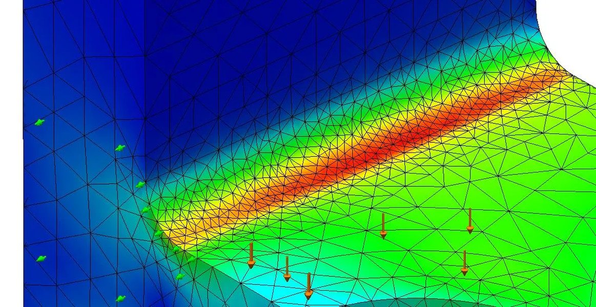
Example of adaptive refinement in a fluid dynamics simulation, where ML could potentially optimize refinement patterns.

Can Machine Learning Truly Revolutionize Finite Element Meshing? Unpacking the Mathematical Proof

Exploring the rigorous mathematical frameworks that demonstrate ML's potential to optimize FEA simulations beyond traditional methods.