
Unveiling the Universe's Electromagnetic Blueprint: Maxwell's Equations and Their Computational Power
Delving into the Fundamental Laws of Electromagnetism and Practical Python Applications
Key Insights into Maxwell's Equations and Their Impact
- Maxwell's Equations as the Foundation of Electromagnetism: These four fundamental equations brilliantly unify electricity and magnetism, providing a comprehensive description of how electric and magnetic fields are generated and interact. They are the bedrock of classical electromagnetism, optics, and electrical engineering, underpinning everything from wireless communication to electric motors.
- Predicting Electromagnetic Waves: One of Maxwell's most profound contributions was the prediction that changing electric and magnetic fields could propagate through space as electromagnetic waves, and that light itself is an electromagnetic phenomenon. This insight revolutionized physics and paved the way for modern communication technologies.
- Solving Maxwell's Equations with Python: Numerical methods, particularly the Finite-Difference Time-Domain (FDTD) method, are widely used to simulate Maxwell's equations. Python, with its extensive libraries and ease of use, has become a powerful tool for implementing these simulations, allowing for the study and visualization of complex electromagnetic phenomena.
Maxwell's Equations stand as one of the most elegant and profound achievements in the history of physics. Developed by James Clerk Maxwell in the 19th century, this set of four partial differential equations describes the behavior of electric and magnetic fields and their interrelationship. They encapsulate a century of experimental observations by scientists like Coulomb, Ampère, and Faraday, synthesizing them into a coherent and unified theory of electromagnetism. These equations are not merely abstract mathematical constructs; they are the instruction manual for how electricity and magnetism work, explaining phenomena ranging from the simplest static charges to the propagation of light and radio waves.
The Four Pillars of Electromagnetism
Maxwell's equations are often presented in two primary forms: the differential form, which describes the fields at a specific point in space and time, and the integral form, which relates fields over regions of space. Both forms convey the same physical laws but are suitable for different types of problems and analytical approaches. The genius of Maxwell was not just in compiling these laws but in adding a crucial term to Ampère's Law, known as the displacement current, which was essential for predicting the existence of electromagnetic waves.
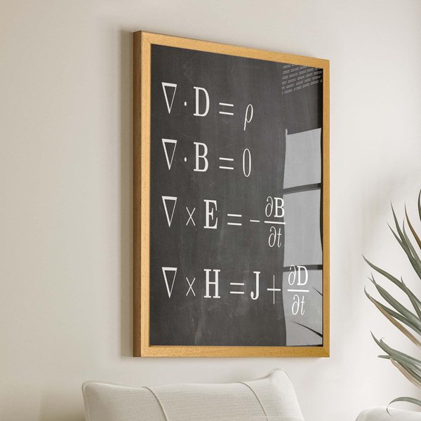
An artistic representation of Maxwell's Equations, highlighting their historical and foundational importance.
A Comprehensive Look at Each Equation
Each of Maxwell's four equations reveals a distinct aspect of electromagnetic behavior:
Gauss's Law for Electricity: The Origin of Electric Fields
This equation, also known as Gauss's Law of Electrostatics, describes the relationship between electric fields and the electric charges that produce them. It states that the electric flux through any closed surface is proportional to the total electric charge enclosed within that surface. Essentially, electric fields diverge from electric charges, meaning positive charges act as sources and negative charges act as sinks for electric field lines.
\[ \oint_S \vec{E} \cdot d\vec{A} = \frac{Q_{\text{enc}}}{\varepsilon_0} \]Where:
- \(\vec{E}\) is the electric field.
- \(d\vec{A}\) is an infinitesimal vector area element on the closed surface \(S\).
- \(Q_{\text{enc}}\) is the total electric charge enclosed by the surface.
- \(\varepsilon_0\) is the permittivity of free space, a fundamental constant.
Gauss's Law for Magnetism: The Absence of Magnetic Monopoles
This law is the magnetic counterpart to Gauss's Law for electricity. It states that the total magnetic flux through any closed surface is always zero. This implies that there are no isolated magnetic poles (magnetic monopoles); magnetic field lines always form continuous loops, without beginning or end. Magnets always have both a north and a south pole.
\[ \oint_S \vec{B} \cdot d\vec{A} = 0 \]Where:
- \(\vec{B}\) is the magnetic field.
- \(d\vec{A}\) is an infinitesimal vector area element on the closed surface \(S\).
Faraday's Law of Induction: Generating Electric Fields from Changing Magnetic Fields
Faraday's Law describes how a changing magnetic field induces an electromotive force (EMF), which in turn creates an electric field. This principle is fundamental to the operation of generators, transformers, and many other electrical devices. It establishes that electric fields are produced by changing magnetic fields.
\[ \oint_C \vec{E} \cdot d\vec{l} = -\frac{d\Phi_B}{dt} \]Where:
- \(\vec{E}\) is the electric field.
- \(d\vec{l}\) is an infinitesimal vector line element along the closed loop \(C\).
- \(\Phi_B\) is the magnetic flux through the surface bounded by the loop \(C\).
- \(-\frac{d\Phi_B}{dt}\) represents the rate of change of magnetic flux, with the negative sign indicating Lenz's Law (the induced current opposes the change in magnetic flux).
Ampère-Maxwell Law: Magnetic Fields from Currents and Changing Electric Fields
This equation, an extension of Ampère's original circuital law, states that circulating magnetic fields can be produced by two sources: electric currents and changing electric fields (Maxwell's displacement current). Maxwell's brilliant addition of the displacement current term was crucial for predicting the existence of electromagnetic waves, as it showed that circulating magnetic fields are produced by changing electric fields and by electric currents.
\[ \oint_C \vec{B} \cdot d\vec{l} = \mu_0 I_{\text{enc}} + \mu_0 \varepsilon_0 \frac{d\Phi_E}{dt} \]Where:
- \(\vec{B}\) is the magnetic field.
- \(d\vec{l}\) is an infinitesimal vector line element along the closed loop \(C\).
- \(\mu_0\) is the permeability of free space.
- \(I_{\text{enc}}\) is the total electric current enclosed by the loop.
- \(\Phi_E\) is the electric flux through the surface bounded by the loop \(C\).
- \(\mu_0 \varepsilon_0 \frac{d\Phi_E}{dt}\) is the displacement current term, representing the contribution of a changing electric field to the magnetic field.
The Unification of Light and Electromagnetism
Perhaps Maxwell's most revolutionary insight was the realization that these four equations could be combined to form a wave equation for both electric and magnetic fields. This wave equation predicted that electromagnetic disturbances could propagate through a vacuum at a constant speed, which Maxwell calculated to be astonishingly close to the known speed of light. This led to the profound conclusion that light itself is an electromagnetic wave.
This Crash Course Physics video provides an accessible explanation of Maxwell's Equations and their significance, including the prediction of electromagnetic waves.
This video, "Maxwell's Equations: Crash Course Physics #37," beautifully illustrates the historical context and the immense impact of Maxwell's work. It highlights how Maxwell synthesized the discoveries of his predecessors and, through his mathematical genius, not only unified electricity and magnetism but also unveiled the electromagnetic nature of light. The concept of electromagnetic waves, propagating through space even without a medium, was a radical departure from previous theories and laid the groundwork for virtually all modern communication technologies, from radio to Wi-Fi.
Comparing Forms: Integral vs. Differential
Maxwell's equations can be expressed in integral form, which describes the behavior of fields over large regions or surfaces, and differential form, which describes the fields at a specific point in space. While physically equivalent, each form has its advantages in different contexts of analysis and problem-solving.
| Law | Description | Integral Form | Differential Form |
|---|---|---|---|
| Gauss's Law for Electricity | Relates the electric field to the distribution of electric charges. Electric field lines originate from positive charges and terminate on negative charges. | \( \oint_S \vec{E} \cdot d\vec{A} = \frac{Q_{\text{enc}}}{\varepsilon_0} \) | \( \nabla \cdot \vec{D} = \rho \) (where \( \vec{D} = \varepsilon_0 \vec{E} \) in vacuum) |
| Gauss's Law for Magnetism | States that magnetic monopoles do not exist; magnetic field lines always form closed loops, with no sources or sinks. | \( \oint_S \vec{B} \cdot d\vec{A} = 0 \) | \( \nabla \cdot \vec{B} = 0 \) |
| Faraday's Law of Induction | Describes how a changing magnetic field induces an electric field (and thus an EMF). This is the principle behind electric generators. | \( \oint_C \vec{E} \cdot d\vec{l} = -\frac{d\Phi_B}{dt} \) | \( \nabla \times \vec{E} = -\frac{\partial \vec{B}}{\partial t} \) |
| Ampère-Maxwell Law | States that magnetic fields are generated by electric currents and by changing electric fields (displacement current). This term was Maxwell's crucial addition. | \( \oint_C \vec{B} \cdot d\vec{l} = \mu_0 I_{\text{enc}} + \mu_0 \varepsilon_0 \frac{d\Phi_E}{dt} \) | \( \nabla \times \vec{H} = \vec{J} + \frac{\partial \vec{D}}{\partial t} \) (where \( \vec{H} = \frac{1}{\mu_0} \vec{B} \) and \( \vec{D} = \varepsilon_0 \vec{E} \) in vacuum) |
Simulating Electromagnetism with Python
Solving Maxwell's equations analytically is often challenging for complex geometries or time-varying fields. This is where numerical methods and computational tools become indispensable. Python, with its rich ecosystem of scientific libraries, offers robust capabilities for simulating electromagnetic phenomena based on Maxwell's equations. The Finite-Difference Time-Domain (FDTD) method is particularly popular for this purpose.
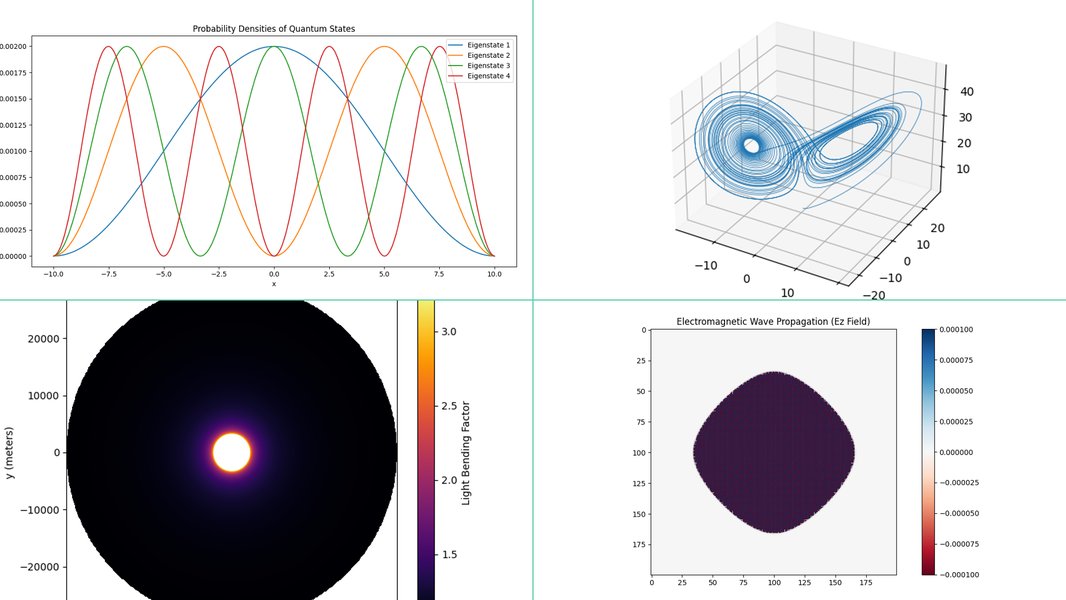
Python code snippet for simulating physics equations, often used for visualizing fields.
Python's Role in Electromagnetic Simulations
Python's appeal for electromagnetic simulations stems from several factors:
- Ease of Use: Python's clear syntax and readability make it accessible for both seasoned researchers and students.
- Extensive Libraries: Libraries like NumPy for numerical operations, SciPy for scientific computing, and Matplotlib for visualization are essential. More specialized packages exist for FDTD simulations, such as GMES and MacroMax.
- Community Support: A large and active community contributes to and supports various physics and engineering simulation packages.
Finite-Difference Time-Domain (FDTD) Method in Python
The FDTD method is a powerful numerical technique for solving Maxwell's equations. It discretizes space and time, approximating derivatives with finite differences. This allows for the calculation of electric and magnetic fields at successive time steps throughout a computational domain.
Here's a conceptual Python code structure for a 1D FDTD simulation of Maxwell's equations. This example focuses on the core update equations, demonstrating how changing electric fields generate magnetic fields and vice versa, leading to wave propagation. For simplicity, we'll consider a vacuum without sources.
# Conceptual 1D FDTD Simulation in Python

import numpy as np
import matplotlib.pyplot as plt
from matplotlib.animation import FuncAnimation

# Constants (normalized for simplicity)
c0 = 1.0  # Speed of light in vacuum
mu0 = 1.0 # Permeability of free space
eps0 = 1.0 # Permittivity of free space

# Simulation parameters
nx = 200     # Number of spatial cells
dx = 0.01    # Spatial step size
dt = dx / c0 # Time step size (CFL condition)
nt = 500     # Number of time steps

# Initialize fields
Ez = np.zeros(nx) # Electric field (z-component)
Hy = np.zeros(nx - 1) # Magnetic field (y-component)

# Source (Gaussian pulse)
source_pos = nx // 2
pulse_width = 10
time_delay = 50

# Store field history for animation
ez_history = []

# FDTD simulation loop
for t in range(nt):
    # Update magnetic field (Hy) using Faraday's Law (nabla x E = -dB/dt)
    # Hy[i+0.5] from Ez[i] and Ez[i+1]
    Hy[:] = Hy[:] - (dt / (mu0 * dx)) * (Ez[1:] - Ez[:-1])

    # Update electric field (Ez) using Ampere-Maxwell Law (nabla x H = dD/dt + J)
    # Ez[i] from Hy[i-0.5] and Hy[i+0.5]
    Ez[1:-1] = Ez[1:-1] - (dt / (eps0 * dx)) * (Hy[1:] - Hy[:-1])

    # Add source (Gaussian pulse)
    Ez[source_pos] += np.exp(-((t - time_delay) / pulse_width)**2)

    # Store current Ez state
    ez_history.append(np.copy(Ez))

# --- Visualization (using Matplotlib for animation) ---
fig, ax = plt.subplots()
line, = ax.plot(np.arange(nx) * dx, ez_history[0], color='#cc9900') # Match H1 color

ax.set_xlim(0, nx * dx)
ax.set_ylim(-1.5, 1.5)
ax.set_xlabel("Position (m)")
ax.set_ylabel("Electric Field (Ez)")
ax.set_title("1D FDTD Simulation of Electromagnetic Wave")
ax.grid(True)

def animate(frame):
    line.set_ydata(ez_history[frame])
    return line,

ani = FuncAnimation(fig, animate, frames=len(ez_history), interval=20, blit=True)
# To save the animation, you might need ffmpeg installed:
# ani.save('em_wave_1d_fdtd.gif', writer='pillow', fps=30)
plt.show()
This code illustrates the fundamental update equations. In a real-world FDTD simulation, more complex boundary conditions, material properties, and source definitions would be incorporated. Libraries like GMES are built upon these principles, offering more advanced and optimized solutions for 2D and 3D simulations.
Understanding the Interplay: A Radar Chart Perspective
Maxwell's equations are not isolated laws but are deeply interconnected, describing a unified electromagnetic force. This radar chart visualizes the conceptual "strength" or "focus" of each equation across key electromagnetic concepts, offering an intuitive grasp of their roles.
The radar chart illustrates how each of Maxwell's equations contributes uniquely to our understanding of electromagnetism. Gauss's Law for Electricity (yellow) excels in describing the fundamental relationship between static charges and electric fields, while Gauss's Law for Magnetism (green) primarily defines the topological nature of magnetic fields, emphasizing the non-existence of magnetic monopoles. Faraday's Law (light green) demonstrates its strength in explaining how changing magnetic fields induce electric fields, linking dynamic phenomena. The Ampère-Maxwell Law (gray) shows high scores in both current-field generation and, crucially, in enabling the concept of wave propagation due to the displacement current term. This visual representation underscores the collective power of these equations in painting a complete picture of electromagnetic interactions, culminating in the prediction of electromagnetic waves.
Applications and Significance
The profound implications of Maxwell's equations extend far beyond theoretical physics. They are the mathematical bedrock for virtually every modern electrical and optical technology. From the design of antennas, optical fibers, and microwave circuits to the principles governing lasers and radar systems, these equations are indispensable. Their ability to predict electromagnetic waves also led directly to the development of radio, television, and all forms of wireless communication that define our digital age.
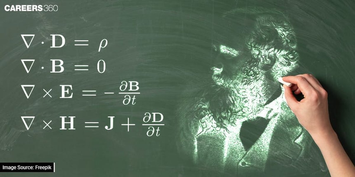
Maxwell's equations, often presented with complex mathematical notation.
Furthermore, Maxwell's equations demonstrated that space and time are inextricably linked in electromagnetic phenomena, paving the way for Einstein's theory of special relativity. The constancy of the speed of light, derived directly from these equations, became a cornerstone of relativistic physics. In essence, Maxwell's work didn't just unify electricity and magnetism; it provided a blueprint for understanding light and laid crucial groundwork for modern physics.
Frequently Asked Questions (FAQ)
What is the main purpose of Maxwell's equations?
Did Maxwell invent all four equations?
Why is the displacement current term so important?
What are the practical applications of Maxwell's equations?
Conclusion
Maxwell's Equations are more than just a collection of formulas; they are a profound testament to the unifying power of physics. By bringing together seemingly disparate phenomena of electricity, magnetism, and light, James Clerk Maxwell provided a single, elegant framework that continues to underpin much of our technological world. Their enduring relevance, from predicting wireless communication to enabling advanced computational simulations, cements their status as cornerstones of scientific understanding. Whether explored through theoretical analysis or practical Python implementations, these equations continue to inspire and drive innovation in science and engineering.
Recommended Further Exploration
- Explore an intuitive understanding of divergence and curl, the mathematical language of Maxwell's equations.
- Learn more about the Finite-Difference Time-Domain (FDTD) method for simulating electromagnetic waves.
- Delve into the historical context and revolutionary impact of Maxwell's unification of electricity and magnetism.
- Discover the myriad applications of electromagnetic waves in contemporary technology, from communication to medical imaging.