
Unlocking the Universe: Maxwell's Equations and Their Pythonic Symphony
Delve into the fundamental laws of electromagnetism and explore their computational realization through Python.
Key Insights into Electromagnetism and Python Simulation
- Maxwell's Equations are the cornerstone of classical electromagnetism: Comprising four fundamental partial differential equations, they comprehensively describe how electric and magnetic fields interact with charges and currents, unifying phenomena like light, radio waves, and electrical circuits.
- Integral and Differential Forms offer versatile perspectives: These equations can be expressed in both integral (describing field behavior over volumes and surfaces) and differential (detailing field variations at specific points) forms, providing flexibility for theoretical analysis and practical applications.
- Numerical methods like FDTD are crucial for real-world simulation: Given the complexity of analytical solutions for many practical scenarios, computational techniques such as the Finite-Difference Time-Domain (FDTD) method, often implemented in Python, are indispensable for simulating electromagnetic phenomena.
The Pillars of Electromagnetism: A Deep Dive into Maxwell's Equations
Maxwell's equations, a monumental achievement in physics, encapsulate the entirety of classical electromagnetism. They elegantly unify previously disparate laws of electricity and magnetism, providing a coherent framework for understanding how electric and magnetic fields are generated, how they interact, and how they propagate through space. These four equations are the foundation for a vast array of modern technologies, from wireless communication and optical fibers to power generation and medical imaging.
The Four Fundamental Laws Explained
Each of Maxwell's four equations addresses a specific aspect of electromagnetic fields, describing relationships between electric fields (\(\mathbf{E}\)), magnetic fields (\(\mathbf{B}\)), charge density (\(\rho\)), and current density (\(\mathbf{J}\)). They are typically presented in both integral and differential forms, each offering a unique perspective on the physical phenomena involved.
Gauss's Law for Electric Fields: The Source of Electric Fields
This law describes how electric charges create electric fields. It states that the total electric flux out of any closed surface is proportional to the total electric charge enclosed within that surface. This implies that electric field lines originate from positive charges and terminate on negative charges.
\[ \text{Differential Form: } \nabla \cdot \mathbf{E} = \frac{\rho}{\varepsilon_0} \] \[ \text{Integral Form: } \oint_S \mathbf{E} \cdot d\mathbf{A} = \frac{Q_{\text{enc}}}{\varepsilon_0} \]Where \(\varepsilon_0\) is the permittivity of free space, \(S\) is a closed surface, \(d\mathbf{A}\) is a differential area vector, and \(Q_{\text{enc}}\) is the total charge enclosed.
Gauss's Law for Magnetic Fields: The Absence of Magnetic Monopoles
This equation, often considered the simplest of the four, states that the total magnetic flux through any closed surface is always zero. This profound implication means that magnetic monopoles (isolated north or south poles) do not exist; magnetic field lines always form continuous closed loops, originating from and terminating on each other.
\[ \text{Differential Form: } \nabla \cdot \mathbf{B} = 0 \] \[ \text{Integral Form: } \oint_S \mathbf{B} \cdot d\mathbf{A} = 0 \]Faraday's Law of Induction: The Genesis of Induced Electric Fields
Faraday's Law details how a changing magnetic field can induce an electric field. This principle is fundamental to the operation of countless electrical devices, including generators, transformers, and induction cooktops. The induced electric field creates a voltage (electromotive force) that can drive currents.
\[ \text{Differential Form: } \nabla \times \mathbf{E} = -\frac{\partial \mathbf{B}}{\partial t} \] \[ \text{Integral Form: } \oint_C \mathbf{E} \cdot d\mathbf{l} = -\frac{d\Phi_B}{dt} \]Here, \(t\) is time, \(C\) is a closed loop, \(d\mathbf{l}\) is a differential path vector, and \(\Phi_B\) is the magnetic flux through the surface bounded by the loop.
Ampère-Maxwell Law: Currents and Changing Electric Fields as Magnetic Sources
Ampère's original law related circulating magnetic fields solely to electric currents. Maxwell's crucial addition of the "displacement current" term, \(\mu_0 \varepsilon_0 \frac{\partial \mathbf{E}}{\partial t}\), completed the set of equations. This term describes how a changing electric field also acts as a source of a magnetic field, just like a real current. This addition was pivotal, as it predicted the existence of self-propagating electromagnetic waves, which travel at the speed of light.
\[ \text{Differential Form: } \nabla \times \mathbf{B} = \mu_0 \mathbf{J} + \mu_0 \varepsilon_0 \frac{\partial \mathbf{E}}{\partial t} \] \[ \text{Integral Form: } \oint_C \mathbf{B} \cdot d\mathbf{l} = \mu_0 I_{\text{enc}} + \mu_0 \varepsilon_0 \frac{d\Phi_E}{dt} \]Where \(\mu_0\) is the permeability of free space, \(I_{\text{enc}}\) is the enclosed current, and \(\Phi_E\) is the electric flux through the surface bounded by the loop.
Maxwell's Equations at a Glance: A Comprehensive Table
The table below provides a concise summary of Maxwell's four equations, detailing their names, mathematical forms (differential and integral), and their profound physical meanings. This synthesis highlights their central role in describing the fundamental nature of electromagnetic phenomena.
| Equation Name | Differential Form | Integral Form | Physical Meaning |
|---|---|---|---|
| Gauss's Law (Electric) | \(\nabla \cdot \mathbf{E} = \frac{\rho}{\varepsilon_0}\) | \(\oint_S \mathbf{E} \cdot d\mathbf{A} = \frac{Q_{\text{enc}}}{\varepsilon_0}\) | Electric charges are the sources/sinks of electric fields. |
| Gauss's Law (Magnetic) | \(\nabla \cdot \mathbf{B} = 0\) | \(\oint_S \mathbf{B} \cdot d\mathbf{A} = 0\) | Magnetic monopoles do not exist; magnetic field lines are always closed loops. |
| Faraday's Law of Induction | \(\nabla \times \mathbf{E} = -\frac{\partial \mathbf{B}}{\partial t}\) | \(\oint_C \mathbf{E} \cdot d\mathbf{l} = -\frac{d\Phi_B}{dt}\) | A changing magnetic field induces an electric field. |
| Ampère–Maxwell Law | \(\nabla \times \mathbf{B} = \mu_0 \mathbf{J} + \mu_0 \varepsilon_0 \frac{\partial \mathbf{E}}{\partial t}\) | \(\oint_C \mathbf{B} \cdot d\mathbf{l} = \mu_0 I_{\text{enc}} + \mu_0 \varepsilon_0 \frac{d\Phi_E}{dt}\) | Electric currents and changing electric fields produce magnetic fields. |
Simulating Electromagnetism with Python: Bridging Theory and Application
While the mathematical elegance of Maxwell's equations is undeniable, obtaining analytical solutions for complex, real-world scenarios is often intractable. This is where numerical methods and powerful programming languages like Python become indispensable. Python's extensive ecosystem of scientific computing libraries makes it an ideal tool for simulating electromagnetic phenomena, from wave propagation to field interactions in intricate geometries.
Key Numerical Methods for Solving Maxwell's Equations
Simulating Maxwell's equations typically involves discretizing space and time and applying numerical approximations to their differential forms. Several methods are widely used, each with its strengths:
Finite-Difference Time-Domain (FDTD) Method
The FDTD method is one of the most popular numerical techniques for solving Maxwell's equations. It directly solves the time-dependent Maxwell's curl equations by discretizing both space and time into a grid. This method is particularly well-suited for simulating transient electromagnetic phenomena, such as wave propagation, scattering, and antenna radiation. Its explicit time-marching scheme makes it computationally efficient for many problems.
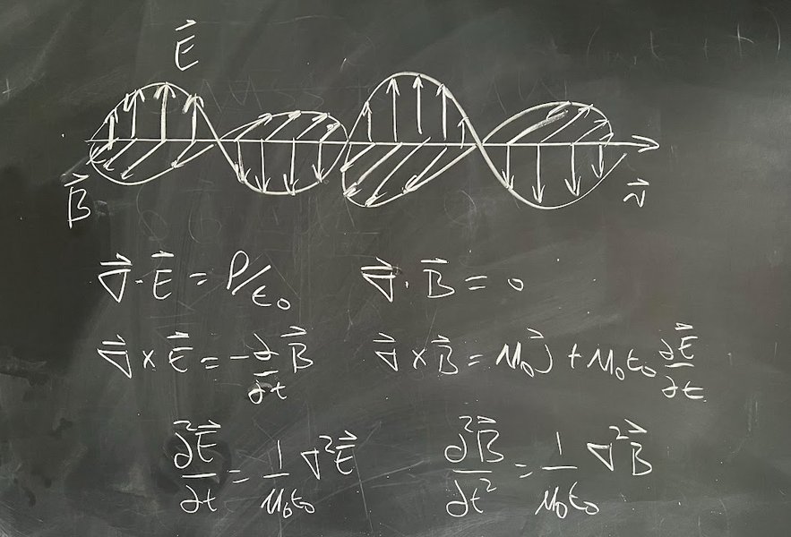
An illustration depicting the propagation of electromagnetic waves, a direct consequence of Maxwell's equations.
Finite Element Method (FEM)
FEM is a powerful numerical technique for solving partial differential equations over complex geometries. In computational electromagnetics, FEM is highly effective for problems involving intricate structures, inhomogeneous materials, and multimodal fields. It discretizes the domain into small elements (e.g., triangles or tetrahedra) and approximates the field within each element using basis functions. FEM is often preferred for frequency-domain analysis and static field problems.
Method of Moments (MoM) / Boundary Element Method (BEM)
These integral equation-based methods are particularly effective for problems involving electrically large structures or those where only the fields on the boundaries are of interest. MoM and BEM convert the differential equations into integral equations that are then solved numerically. They are often used for antenna design, scattering analysis, and interconnect modeling.
Illustrative Python Code: A 2D FDTD Simulation Snippet
The following Python code snippet demonstrates the core principles of a 2D FDTD simulation for Maxwell's equations. This example focuses on the time-evolution of electric and magnetic fields on a grid, illustrating how the curl equations are numerically updated. While simplified, it provides a foundational understanding of how these powerful simulations are constructed using basic Python libraries like NumPy.
import numpy as np

# Simulation parameters
nx, ny = 101, 101            # Grid size in x and y
dx = dy = 1e-3              # Spatial step (meters)
c = 299792458               # Speed of light in vacuum (m/s)
dt = dx / (2 * c)           # Time step (Courant stability condition)
steps = 200                 # Number of time steps for the simulation

# Initialize field arrays (Ez for electric field, Hx/Hy for magnetic fields)
Ez = np.zeros((nx, ny))     # z-component of electric field
Hx = np.zeros((nx, ny))     # x-component of magnetic field
Hy = np.zeros((nx, ny))     # y-component of magnetic field

# Constants for free space
MU0 = 4 * np.pi * 1e-7      # Permeability of free space
EPSILON0 = 8.854e-12        # Permittivity of free space

# Source parameters - a simple Gaussian pulse applied at the center
source_position = (nx // 2, ny // 2)
source_time = 0
def gaussian_pulse(t, t0, sigma):
    return np.exp(-((t - t0) / sigma)**2)

# FDTD simulation loop
for n in range(steps):
    # Update magnetic field (Hx, Hy) based on Faraday's Law
    # Hx update (approximation of -1/mu0 * dEz/dy)
    # The negative sign in Faraday's law accounts for the direction of induction.
    Hx[:, :-1] = Hx[:, :-1] - (dt / (MU0 * dy)) * (Ez[:, 1:] - Ez[:, :-1])

    # Hy update (approximation of 1/mu0 * dEz/dx)
    Hy[:-1, :] = Hy[:-1, :] + (dt / (MU0 * dx)) * (Ez[1:, :] - Ez[:-1, :])

    # Apply boundary conditions for Hx and Hy (simplified, often PML or ABCs are used)
    # For a full simulation, absorbing boundary conditions (ABCs) or perfectly matched layers (PMLs)
    # would be implemented here to prevent reflections from the grid edges.

    # Update electric field (Ez) based on Ampere-Maxwell Law
    # Ez update (approximation of 1/epsilon0 * (dHy/dx - dHx/dy))
    Ez[1:-1, 1:-1] = Ez[1:-1, 1:-1] + (dt / (EPSILON0 * dx)) * \
                     ((Hy[1:-1, 1:-1] - Hy[:-2, 1:-1]) - \
                      (Hx[1:-1, 1:-1] - Hx[1:-1, :-2]))

    # Source injection: Add a Gaussian pulse at a specific point
    Ez[source_position] += gaussian_pulse(source_time, 30, 10)
    source_time += 1 # Increment source time for pulse evolution

    # Apply boundary conditions for Ez (e.g., PEC, PMC, or ABCs)
    # Similar to H-fields, proper boundary conditions are crucial for accurate simulations.

    # In a full simulation, you would typically save or visualize the fields at certain intervals
    # print(f"Time step: {n+1}, Max Ez: {np.max(Ez)}")

print("Simulation complete. Field values are in Ez, Hx, Hy arrays.")
This code illustrates the iterative nature of FDTD, where electric and magnetic fields are updated in alternating half-steps using their spatial differences. The Gaussian pulse serves as a simple source to initiate wave propagation. For robust, production-level simulations, more advanced aspects like absorbing boundary conditions (e.g., perfectly matched layers or Mur absorbing boundary conditions) are essential to prevent unphysical reflections from the simulation boundaries.
Python Libraries and Tools for Advanced Electromagnetic Simulations
Beyond basic implementations, several specialized Python packages and frameworks exist to facilitate more complex and efficient electromagnetic simulations:
- macromax: This package is designed to solve macroscopic Maxwell's equations within complex dielectric materials. It is particularly useful for scenarios involving heterogeneous, anisotropic, and magnetic media, making it valuable for light propagation studies in various materials.
- GMES (GIST Maxwell's Equations Solver): An open-source Python package that provides a robust implementation of the FDTD method. It emphasizes an object-oriented design, promoting well-structured and extensible code for simulating Maxwell's equations.
- PyCharge: A computational electrodynamics simulator that calculates electromagnetic fields and potentials generated by moving point charges. Unlike grid-based methods, PyCharge leverages analytical solutions for individual point charges to compute the overall field.
- fdtd: A comprehensive 3D electromagnetic FDTD simulator written in Python, offering an optional PyTorch backend for leveraging GPU acceleration, which significantly speeds up large-scale simulations.
- py-maxwell-fd3d: A Python implementation focusing on the 3D curl-curl E-field equations from Maxwell's equations, tailored for efficient finite-difference simulations.
- Ceviche: This tool provides core electromagnetic simulation capabilities, primarily using NumPy and SciPy, and is notable for its integration with automatic differentiation frameworks, useful for inverse design problems.
- gprMax: While primarily developed for Ground Penetrating Radar (GPR) modeling, gprMax is a powerful FDTD-based software written in Python (with performance-critical parts in Cython/OpenMP) that can be adapted for a broader range of electromagnetic wave propagation applications.
Visualizing Key Aspects of Maxwell's Equations
Understanding the interplay between electric and magnetic fields, and how different factors influence their behavior, can be challenging. A radar chart offers a visual way to compare how various aspects of Maxwell's equations contribute to different electromagnetic phenomena or simulation characteristics. While the data points are illustrative and based on qualitative assessment, this chart highlights the relative importance of different components for a given context.
Radar chart illustrating the conceptual influence of different Maxwell's equation terms on various electromagnetic phenomena and simulation attributes. Higher values indicate greater relevance or contribution.
The Interconnected World of Electromagnetic Concepts
Maxwell's equations are not isolated formulas; they are part of a rich tapestry of concepts that define electromagnetism. This mindmap illustrates the interconnectedness of key ideas related to Maxwell's equations, from their fundamental components and implications to the numerical methods and Python tools used for their simulation.
Understanding Maxwell's Equations with Visual Aids
To further solidify your understanding of Maxwell's equations and their practical application in simulation, this video provides an excellent introduction to developing a 1D FDTD program using Python. It demystifies the process of translating these fundamental equations into a computational model, showing how electric and magnetic fields can be numerically updated over time to simulate wave propagation.
This video, titled "Write your own 1D - FDTD program with python," demonstrates the core principles of implementing Maxwell's equations in one dimension using the Finite Difference Time Domain method. It's an invaluable resource for understanding the practical steps involved in computational electromagnetics.
The video walks you through the fundamental steps of creating a simple 1D FDTD simulator, which is a foundational skill for anyone looking to delve into more complex electromagnetic simulations. It visually explains how the electric and magnetic fields are staggered in space and time, and how their interactions are modeled using finite differences, directly reflecting Faraday's and Ampere-Maxwell's laws. This hands-on approach is crucial for gaining an intuitive grasp of how abstract mathematical equations translate into dynamic physical phenomena.
Frequently Asked Questions (FAQ)
Conclusion: The Enduring Legacy of Electromagnetism
Maxwell's equations stand as a testament to the unifying power of physics, knitting together the seemingly disparate phenomena of electricity and magnetism into a single, elegant theory. These four partial differential equations not only provide a complete description of classical electromagnetic fields but also laid the groundwork for modern physics, directly leading to the understanding of light as an electromagnetic wave and forming the bedrock of wireless communication, optics, and countless other technological advancements. The ability to express these laws in both integral and differential forms underscores their versatility for different analytical contexts. Furthermore, the advent of computational tools and programming languages like Python has revolutionized the study and application of electromagnetism. Numerical methods such as FDTD, FEM, and MoM allow engineers and physicists to simulate complex electromagnetic scenarios that defy analytical solutions. The vibrant ecosystem of Python libraries, including specialized packages like macromax, GMES, and fdtd, empowers researchers and developers to explore, design, and innovate in areas ranging from antenna design and photonics to bioelectromagnetics. As our technological landscape continues to evolve, the fundamental principles enshrined in Maxwell's equations, coupled with the power of modern computation, will remain indispensable for driving future discoveries and innovations.
Recommended Further Exploration
- Explore a detailed derivation of Maxwell's equations from fundamental principles.
- Investigate advanced numerical methods and their applications in electromagnetics.
- Discover various modern technological applications that are built upon Maxwell's equations.
- Learn more about computational electromagnetics with a focus on Python-based tools and tutorials.