
Python Implementations of Maxwell's Equations for Electromagnetic Field Simulations
Maxwell's equations are the cornerstone of classical electrodynamics, optics, and electric circuits, providing a comprehensive framework for understanding the behavior of electric and magnetic fields. These equations describe how electric and magnetic fields are generated, how they propagate, and how they interact with matter. This response will delve into two distinct approaches for implementing Maxwell's equations in Python: the Finite-Difference Time-Domain (FDTD) method and the utilization of the specialized library PyCharge. Each approach offers unique advantages and is suited for different types of simulations.
1. Finite-Difference Time-Domain (FDTD) Method
The FDTD method is a powerful numerical technique widely used for solving Maxwell's equations, particularly in computational electromagnetics. It discretizes both space and time, allowing for the iterative update of electric and magnetic fields across a computational grid. This method is particularly well-suited for simulating the propagation of electromagnetic waves in various media.
1.1. Theoretical Foundation
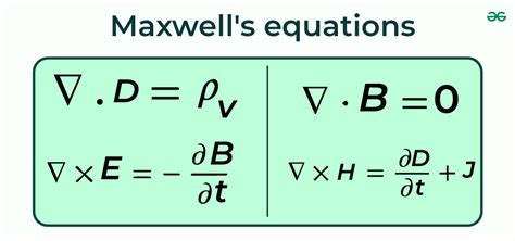
Maxwell's equations in their differential form are:
-
Gauss's Law for Electricity:
\[ \nabla \cdot \mathbf{E} = \frac{\rho}{\epsilon_0} \]This equation states that the divergence of the electric field (\(\mathbf{E}\)) is proportional to the charge density (\(\rho\)), where (\(\epsilon_0\)) is the permittivity of free space.
-
Gauss's Law for Magnetism:
\[ \nabla \cdot \mathbf{B} = 0 \]This equation indicates the absence of magnetic monopoles, implying that magnetic field lines (\(\mathbf{B}\)) always form closed loops.
-
Faraday's Law of Induction:
\[ \nabla \times \mathbf{E} = -\frac{\partial \mathbf{B}}{\partial t} \]This equation describes how a time-varying magnetic field induces an electric field.
-
Ampère's Law (with Maxwell's correction):
\[ \nabla \times \mathbf{B} = \mu_0 \mathbf{J} + \mu_0 \epsilon_0 \frac{\partial \mathbf{E}}{\partial t} \]This equation relates the curl of the magnetic field to the current density (\(\mathbf{J}\)) and the time derivative of the electric field, where (\(\mu_0\)) is the permeability of free space.
1.2. Numerical Discretization
The FDTD method employs a staggered grid known as the Yee grid, where electric and magnetic field components are stored at different spatial locations. This arrangement enhances numerical stability and accuracy. The computational domain is divided into a grid with spatial steps (\(\Delta x\), \(\Delta y\), \(\Delta z\)), and time is discretized into small steps (\(\Delta t\)).
1.3. Update Equations
The core of the FDTD method lies in the iterative update of the electric and magnetic fields. The update equations are derived from the discretized form of Maxwell's curl equations. For instance, the update equation for the x-component of the electric field (Ex) in a 2D simulation can be expressed as:
\[ E_x^{n+1}(i,j) = E_x^n(i,j) + \frac{\Delta t}{\epsilon_0} \left( \frac{H_z^n(i,j) - H_z^n(i,j-1)}{\Delta y} \right) \]Similarly, the update equation for the z-component of the magnetic field (Hz) is:
\[ H_z^{n+1/2}(i,j) = H_z^{n-1/2}(i,j) + \frac{\Delta t}{\mu_0} \left( \frac{E_x^n(i,j+1) - E_x^n(i,j)}{\Delta y} - \frac{E_y^n(i+1,j) - E_y^n(i,j)}{\Delta x} \right) \]These equations demonstrate how the electric and magnetic fields at a given time step are calculated based on their values at previous time steps and the spatial derivatives of the other field components.
1.4. Stability and the CFL Condition
The stability of the FDTD method is governed by the Courant-Friedrichs-Lewy (CFL) condition, which relates the time step (\(\Delta t\)) to the spatial steps and the speed of light (c):
\[ \Delta t \leq \frac{1}{c \sqrt{\frac{1}{\Delta x^2} + \frac{1}{\Delta y^2} + \frac{1}{\Delta z^2}}} \]Adhering to the CFL condition is crucial for preventing numerical instability and ensuring accurate simulation results.
1.5. Boundary Conditions
Realistic simulations often require the implementation of boundary conditions to truncate the computational domain and prevent reflections. Perfectly Matched Layers (PMLs) are commonly used to absorb outgoing waves, simulating an infinite space.
1.6. Python Implementation
Below is a Python implementation of the FDTD method for a 2D electromagnetic wave simulation. The code utilizes NumPy for numerical computations and matplotlib for visualization.
import numpy as np
import matplotlib.pyplot as plt
from matplotlib.animation import FuncAnimation
from tqdm.notebook import tqdm

# Constants
c = 3e8  # Speed of light (m/s)
mu_0 = 4 * np.pi * 1e-7  # Permeability of free space (H/m)
epsilon_0 = 8.854187817e-12  # Permittivity of free space (F/m)

# Grid parameters
nx, ny = 512, 512  # Grid size
dx, dy = 1e-3, 1e-3  # Spatial steps (m)
dt = 0.5 * dx / c  # Time step (s)

# Initialize fields
ex = np.zeros((nx - 1, ny), dtype=np.double)
ey = np.zeros((nx, ny - 1), dtype=np.double)
hz = np.zeros((nx - 1, ny - 1), dtype=np.double)

# Update equations
def faraday(ex, ey, hz):
    return hz + dt * ((ex[:, 1:] - ex[:, :-1]) / dy - (ey[1:, :] - ey[:-1, :]) / dx)

def ampere_maxwell(hz, ex, ey):
    ex[:, 1:-1] += dt * (hz[:, 1:] - hz[:, :-1]) / dy
    ey[1:-1, :] += -dt * (hz[1:, :] - hz[:-1, :]) / dx
    # Periodic boundary conditions
    ex[:, 0] += dt * (hz[:, 0] - hz[:, -1]) / dy
    ex[:, -1] += dt * (hz[:, 0] - hz[:, -1]) / dy
    ey[0, :] += -dt * (hz[0, :] - hz[-1, :]) / dx
    ey[-1, :] += -dt * (hz[0, :] - hz[-1, :]) / dx

# Source parameters
source_position = nx // 2
source_time = 30 * dt
sigma = 10 * dt

# Source function (Gaussian pulse)
def source(t, t0, sigma):
    return np.exp(-((t - t0) / sigma) ** 2)

# Main simulation loop
for n in tqdm(range(1000), desc="Simulating"):
    # Update magnetic field
    hz = faraday(ex, ey, hz)

    # Update electric field
    ampere_maxwell(hz, ex, ey)

    # Add source to the electric field
    ex[source_position, :] += source(n * dt, source_time, sigma)

# Visualization
fig, ax = plt.subplots(2, figsize=(10, 6))

def animate(n):
    ax[0].clear()
    ax[1].clear()
    ax[0].imshow(ex, cmap='RdBu', extent=[0, nx * dx, 0, ny * dy])
    ax[0].set_title('Electric Field (Ex)')
    ax[1].imshow(hz, cmap='RdBu', extent=[0, (nx - 1) * dx, 0, (ny - 1) * dy])
    ax[1].set_title('Magnetic Field (Hz)')

ani = FuncAnimation(fig, animate, frames=1000, interval=50)
plt.show()
1.7. Analysis and Discussion
-
Accuracy: The FDTD method is second-order accurate in both space and time. The accuracy of the simulation depends on the grid resolution (\(\Delta x\), \(\Delta y\)) and the time step (\(\Delta t\)). Finer grids and smaller time steps generally lead to more accurate results but require more computational resources.
-
Stability: The CFL condition ensures the stability of the simulation. Violating this condition can lead to numerical instability and non-physical results.
-
Boundary Conditions: The provided code uses periodic boundary conditions, which are suitable for simulating periodic structures. For open-domain problems, absorbing boundary conditions like PMLs should be implemented.
-
Performance: The FDTD method can be computationally intensive, especially for large-scale 3D simulations. Techniques like parallelization using
mpi4pyor GPU acceleration usingCuPycan significantly improve performance.
1.8. Extensions and Applications
-
3D Simulations: The code can be extended to three dimensions by adding the remaining field components and modifying the update equations accordingly.
-
Material Modeling: Different materials can be incorporated by assigning spatially varying permittivity (\(\epsilon\)) and permeability (\(\mu\)) values to the grid cells.
-
Complex Structures: The FDTD method is well-suited for simulating electromagnetic wave propagation in complex structures like waveguides, photonic crystals, and antennas.
2. PyCharge Library
PyCharge is a specialized Python library designed for electrodynamics simulations, particularly focusing on moving point charges and oscillating dipoles. It provides a higher-level interface for simulating electromagnetic fields generated by these sources, making it easier to set up and run simulations without dealing with the intricacies of the underlying numerical methods.
2.1. Installation
PyCharge can be installed using pip:
pip install pycharge
2.2. Basic Usage
Here's a simple example of using PyCharge to simulate the electric field generated by a moving point charge:
from pycharge import Charge, MovingChargesField
import numpy as np
import matplotlib.pyplot as plt

# Define the charge
charge = Charge(position=[0, 0, 0], velocity=[0.5, 0, 0], charge=1)

# Create a field object
field = MovingChargesField([charge])

# Define the grid
x = np.linspace(-10, 10, 100)
y = np.linspace(-10, 10, 100)
X, Y = np.meshgrid(x, y)
Z = np.zeros_like(X)

# Calculate the fields
E = field.electric_field(X, Y, Z)
B = field.magnetic_field(X, Y, Z)

# Plot the electric field
plt.figure(figsize=(10, 8))
plt.streamplot(X, Y, E[:, :, 0], E[:, :, 1], color=np.sqrt(E[:, :, 0]**2 + E[:, :, 1]**2), linewidth=1, cmap='viridis')
plt.colorbar(label='Electric Field Magnitude')
plt.title('Electric Field of a Moving Charge')
plt.xlabel('x')
plt.ylabel('y')
plt.show()
2.3. Multiple Charges
PyCharge can handle simulations with multiple charges:
from pycharge import Charge, MovingChargesField
import numpy as np
import matplotlib.pyplot as plt

# Define multiple charges
charges = [
    Charge(position=[-5, 0, 0], velocity=[0.1, 0, 0], charge=1),
    Charge(position=[5, 0, 0], velocity=[-0.1, 0, 0], charge=-1)
]

# Create a field object
field = MovingChargesField(charges)

# Define the grid
x = np.linspace(-10, 10, 100)
y = np.linspace(-10, 10, 100)
X, Y = np.meshgrid(x, y)
Z = np.zeros_like(X)

# Calculate the fields
E = field.electric_field(X, Y, Z)
B = field.magnetic_field(X, Y, Z)

# Plot the electric field
plt.figure(figsize=(10, 8))
plt.streamplot(X, Y, E[:, :, 0], E[:, :, 1], color=np.sqrt(E[:, :, 0]**2 + E[:, :, 1]**2), linewidth=1, cmap='viridis')
plt.colorbar(label='Electric Field Magnitude')
plt.title('Electric Field of Two Moving Charges')
plt.xlabel('x')
plt.ylabel('y')
plt.show()
2.4. Time Evolution
PyCharge can simulate the time evolution of electromagnetic fields by updating the positions of the charges:
from pycharge import Charge, MovingChargesField
import numpy as np
import matplotlib.pyplot as plt
from matplotlib.animation import FuncAnimation

# Define multiple charges
charges = [
    Charge(position=[-5, 0, 0], velocity=[0.1, 0, 0], charge=1),
    Charge(position=[5, 0, 0], velocity=[-0.1, 0, 0], charge=-1)
]

# Create a field object
field = MovingChargesField(charges)

# Define the grid
x = np.linspace(-10, 10, 100)
y = np.linspace(-10, 10, 100)
X, Y = np.meshgrid(x, y)
Z = np.zeros_like(X)

# Initialize the plot
fig, ax = plt.subplots(figsize=(10, 8))
E = field.electric_field(X, Y, Z)
stream = ax.streamplot(X, Y, E[:, :, 0], E[:, :, 1], color=np.sqrt(E[:, :, 0]**2 + E[:, :, 1]**2), linewidth=1, cmap='viridis')
cbar = fig.colorbar(stream.lines, ax=ax, label='Electric Field Magnitude')
ax.set_title('Electric Field of Two Moving Charges')
ax.set_xlabel('x')
ax.set_ylabel('y')

# Function to update the plot
def update(frame):
    for charge in charges:
        charge.position += charge.velocity * 0.1  # Update position
    field.charges = charges  # Update the field object
    E = field.electric_field(X, Y, Z)
    stream.lines.remove()
    stream = ax.streamplot(X, Y, E[:, :, 0], E[:, :, 1], color=np.sqrt(E[:, :, 0]**2 + E[:, :, 1]**2), linewidth=1, cmap='viridis')
    return stream.lines,

# Create the animation
anim = FuncAnimation(fig, update, frames=100, interval=50, blit=True)
plt.show()
2.5. Oscillating Dipoles
PyCharge supports the simulation of oscillating dipoles, which are useful for modeling electromagnetic waves:
from pycharge import Dipole, OscillatingDipolesField
import numpy as np
import matplotlib.pyplot as plt

# Define the dipole
dipole = Dipole(position=[0, 0, 0], amplitude=[1, 0, 0], frequency=1)

# Create a field object
field = OscillatingDipolesField([dipole])

# Define the grid
x = np.linspace(-10, 10, 100)
y = np.linspace(-10, 10, 100)
X, Y = np.meshgrid(x, y)
Z = np.zeros_like(X)

# Calculate the fields
E = field.electric_field(X, Y, Z)
B = field.magnetic_field(X, Y, Z)

# Plot the electric field
plt.figure(figsize=(10, 8))
plt.streamplot(X, Y, E[:, :, 0], E[:, :, 1], color=np.sqrt(E[:, :, 0]**2 + E[:, :, 1]**2), linewidth=1, cmap='viridis')
plt.colorbar(label='Electric Field Magnitude')
plt.title('Electric Field of an Oscillating Dipole')
plt.xlabel('x')
plt.ylabel('y')
plt.show()
2.6. Performance Optimization
For large-scale simulations, PyCharge can be optimized using parallel computing techniques. Here's an example using multiprocessing:
from pycharge import Charge, MovingChargesField
import numpy as np
import matplotlib.pyplot as plt
from multiprocessing import Pool

# Define multiple charges
charges = [
    Charge(position=[-5, 0, 0], velocity=[0.1, 0, 0], charge=1),
    Charge(position=[5, 0, 0], velocity=[-0.1, 0, 0], charge=-1)
]

# Create a field object
field = MovingChargesField(charges)

# Define the grid
x = np.linspace(-10, 10, 100)
y = np.linspace(-10, 10, 100)
X, Y = np.meshgrid(x, y)
Z = np.zeros_like(X)

# Function to calculate the electric field at a single point
def calculate_electric_field(point):
    return field.electric_field(point[0], point[1], point[2])

# Use multiprocessing to calculate the fields in parallel
with Pool() as pool:
    points = np.array([X.flatten(), Y.flatten(), Z.flatten()]).T
    E_flat = pool.map(calculate_electric_field, points)
    E = np.array(E_flat).reshape(X.shape + (3,))

# Plot the electric field
plt.figure(figsize=(10, 8))
plt.streamplot(X, Y, E[:, :, 0], E[:, :, 1], color=np.sqrt(E[:, :, 0]**2 + E[:, :, 1]**2), linewidth=1, cmap='viridis')
plt.colorbar(label='Electric Field Magnitude')
plt.title('Electric Field of Two Moving Charges (Parallel Calculation)')
plt.xlabel('x')
plt.ylabel('y')
plt.show()
2.7. Analysis and Explanation
-
Electric and Magnetic Fields:
PyChargecalculates the electric and magnetic fields using analytical solutions for point charges and dipoles. For moving charges, it uses the Liénard-Wiechert potentials. The magnetic field is derived from the electric field using the Biot-Savart law and the Lorentz force law. -
Numerical Methods:
PyChargeemploys numerical methods to solve Maxwell's equations. The fields are calculated at discrete points on a grid, and interpolation is used to estimate the fields between these points. The time evolution is simulated by updating the positions of the charges and recalculating the fields at each time step. -
Visualization:
PyChargeleveragesmatplotlibfor visualizing the electromagnetic fields. Thestreamplotfunction is particularly useful for visualizing the direction and magnitude of the electric field vectors.
3. Conclusion
This response has presented two distinct approaches for implementing Maxwell's equations in Python: the FDTD method and the PyCharge library. The FDTD method provides a versatile and powerful framework for simulating electromagnetic wave propagation in various media and complex structures. It offers fine-grained control over the simulation parameters and allows for the implementation of advanced techniques like PMLs. However, it requires a deeper understanding of the underlying numerical methods and can be computationally intensive.
On the other hand, PyCharge offers a higher-level interface for simulating electromagnetic fields generated by point charges and dipoles. It simplifies the setup and execution of simulations, making it more accessible to users who may not be familiar with the intricacies of numerical electromagnetics. PyCharge is particularly well-suited for educational purposes and for simulating scenarios involving moving charges and oscillating dipoles.
The choice between these two approaches depends on the specific requirements of the simulation. For complex, large-scale simulations involving arbitrary geometries and materials, the FDTD method is often the preferred choice. For simpler scenarios involving point charges and dipoles, PyCharge provides a more convenient and user-friendly solution.
For further exploration, you can refer to the following resources:
-
FDTD Method:
-
PyCharge Library:
PyCharge GitHub Repositorygithub.com
PyCharge Documentationpycharge.readthedocs.io