

Key Insights into Probabilistic Simulation
- Monte Carlo Simulation provides a foundational framework for solving complex problems through repeated random sampling, originating from nuclear physics during the Manhattan Project.
- Metropolis-Hastings Algorithm is a general MCMC method that enables sampling from complex probability distributions even when their normalization constant is unknown, making it highly versatile for Bayesian inference and statistical physics.
- Gibbs Sampling is a specialized MCMC technique, often considered a special case of Metropolis-Hastings, particularly effective when conditional distributions of individual variables are easier to sample from.
The realms of statistics, physics, and machine learning have been profoundly reshaped by powerful computational methods that leverage randomness to solve otherwise intractable problems. At the heart of these advancements lie Monte Carlo Simulation, Gibbs Sampling, and the Metropolis-Hastings algorithm. These techniques, though distinct in their specific mechanisms, share a common goal: to explore and understand complex probability distributions, often when direct analytical solutions are elusive.
This comprehensive overview delves into the historical context, fundamental principles, and diverse applications of these methods, complemented by detailed case studies to illustrate their practical impact.
The Genesis of Monte Carlo Simulation: Harnessing Randomness
The term "Monte Carlo" evokes images of a famous casino, and fittingly so, as this method fundamentally relies on random processes. Its origins, however, are rooted in a far more critical endeavor: the Manhattan Project during World War II.
Wartime Innovations and Scientific Breakthroughs
Developed in the 1940s by pioneers such as Stanislaw Ulam and John von Neumann, the Monte Carlo method was a response to the computational challenges of nuclear physics. Researchers faced complex problems related to neutron diffusion and other atomic phenomena that could not be solved using deterministic mathematical approaches. The idea was to approximate solutions by simulating these processes numerous times using random numbers.
 A visual representation highlighting the iterative nature common to Monte Carlo methods.
Core Principles of Monte Carlo Simulation
At its essence, Monte Carlo simulation involves generating repeated random samples from a probability distribution to obtain numerical results. This approach is particularly effective for problems that involve significant uncertainties or are too complex for analytical solutions.
Key Applications Across Disciplines
The versatility of Monte Carlo has led to its adoption in an extensive range of fields:
- Finance and Investment: Used for portfolio risk assessment, option pricing, and market trend prediction.
- Project Management: Evaluating project timelines and costs under various uncertainties.
- Engineering: Simulating complex systems like airflow, structural integrity, and electronic circuits.
- Healthcare: Modeling disease progression, optimizing resource allocation, and simulating radiotherapy.
- Quality Control: Estimating product reliability and failure rates.
- Tokenomics Design: Assessing risk and volatility in cryptocurrency projects.
Monte Carlo methods are broadly categorized into applications for optimization, numerical integration, and non-uniform random variate generation, making them a foundational tool for computational analysis.
Metropolis-Hastings Algorithm: A General MCMC Framework
Building upon the principles of Monte Carlo, the Metropolis-Hastings algorithm offers a more sophisticated approach for sampling from complex probability distributions, especially when direct sampling is not feasible.
From Physics to General Statistical Sampling
The original Metropolis algorithm was introduced in 1953 by Nicholas Metropolis and his colleagues to simulate systems in statistical physics. In 1970, W. K. Hastings generalized this method, giving us the Metropolis-Hastings algorithm. This generalization allowed for asymmetric proposal distributions, significantly broadening its applicability.
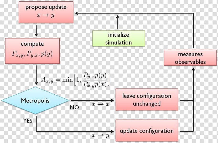
 Flowchart illustrating the steps of the Metropolis-Hastings algorithm for parameter estimation.
Understanding the Metropolis-Hastings Mechanism
The power of Metropolis-Hastings lies in its ability to generate samples from a target distribution even when its functional form is known only up to a constant (i.e., its normalization constant is unknown or difficult to calculate). It operates by proposing new states and then accepting or rejecting them based on an acceptance probability.
- Proposal Distribution (q(x' | x)): This distribution suggests a new candidate state (x') given the current state (x). The choice of this distribution can significantly impact the algorithm's efficiency.
- Acceptance Probability ($\alpha$): A crucial step where the algorithm calculates the probability of moving to the proposed state. This probability depends on the ratio of the target distribution at the proposed and current states, and the proposal distribution probabilities. For a target distribution $p(x)$ and proposal $q(x'|x)$, the acceptance probability is: \[ \alpha(x^*, x_t) = \min \left( 1, \frac{p(x^*) q(x_t | x^*)}{p(x_t) q(x^* | x_t)} \right) \] This ingenious formulation allows sampling from $p(x)$ without knowing its normalizing constant.
- Iterative Process: The algorithm repeatedly proposes states and accepts/rejects them, forming a Markov chain whose stationary distribution is the target distribution.
Applications of Metropolis-Hastings
Metropolis-Hastings is indispensable in:
- Bayesian Statistics: Sampling from posterior distributions, which are often analytically intractable.
- Statistical Physics: Simulating the behavior of complex physical systems.
- Machine Learning: Used in various probabilistic models, particularly for parameter estimation.
Gibbs Sampling: A Specialized MCMC Approach
Gibbs sampling is a specific, highly efficient type of Markov Chain Monte Carlo algorithm, often considered a special case of Metropolis-Hastings. It gained significant popularity in the Bayesian statistics community in the early 1990s.
Leveraging Conditional Distributions
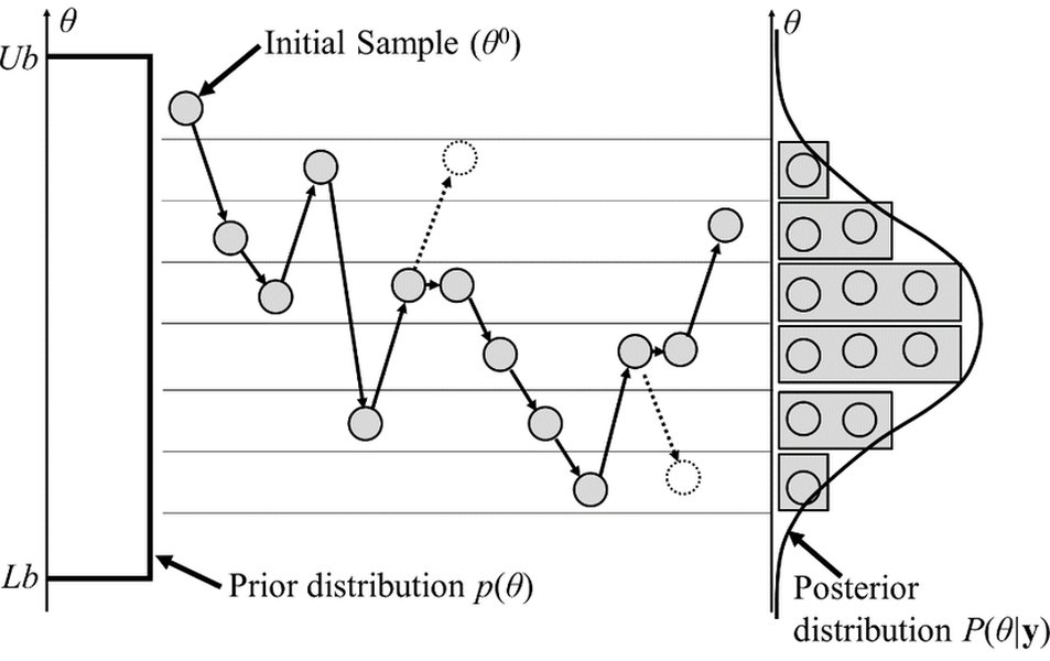
Named after physicist Josiah Willard Gibbs, this method is particularly useful when sampling from a multivariate probability distribution is difficult, but sampling from the conditional distribution of each variable (given the others) is relatively easy. Unlike Metropolis-Hastings, Gibbs sampling generally has an acceptance probability of 1, as it directly samples from the exact conditional distributions.
 An illustration depicting the iterative process of Gibbs sampling within a multi-dimensional parameter space.
How Gibbs Sampling Works
The process is iterative:
- Start with initial values for all variables.
- For each variable, sample a new value from its conditional distribution, given the current values of all other variables.
- Repeat this process for all variables in sequence, cycling through them multiple times.
- After an initial "burn-in" period, the collected samples will approximate the desired joint distribution.
Key Applications of Gibbs Sampling
Gibbs sampling is a cornerstone in:
- Bayesian Inference: Estimating posterior distributions for models with many parameters.
- Computational Statistics: Solving problems where direct calculation of joint distributions is infeasible.
- Machine Learning: Used in models like Latent Dirichlet Allocation (LDA) for topic modeling.
- Image Analysis and Genomics: Analyzing complex data structures where dependencies between variables are crucial.
Mind Map of Interconnected Concepts
To visualize the relationships and hierarchical structure among these concepts, consider the following mind map. It delineates how Monte Carlo simulation forms the broader category, with MCMC methods as a subset, and Gibbs Sampling and Metropolis-Hastings as key algorithms within MCMC.
Deep Dive: Case Studies and Analytical Insights
To appreciate the practical impact of Gibbs Sampling and Metropolis-Hastings, let's examine illustrative case studies that highlight their methodology and analytical power.
Estimating Parameters in a Bayesian Biological Model
Imagine a research scenario in bioinformatics where the goal is to estimate multiple interconnected parameters, such as population sizes and gene frequencies, within a complex biological system. The joint posterior distribution of these parameters is analytically intractable, making direct estimation challenging.
Methodology in Action:
In this context, Gibbs sampling becomes an invaluable tool:
- Model Definition: A probabilistic model is defined, incorporating the unknown parameters (e.g., birth rates, allele frequencies) and linking them to observed biological data.
- Conditional Distributions: The researchers derive the conditional probability distribution for each parameter, assuming the current values of all other parameters are known. This is a critical step, as Gibbs sampling's efficiency relies on these conditional distributions being tractable to sample from.
- Iterative Sampling: The algorithm begins with arbitrary initial values for all parameters. It then iteratively samples each parameter from its conditional distribution. For example, it might sample parameter $\theta_1$ given $\theta_2, \theta_3, \dots, \theta_k$, then sample $\theta_2$ given the newly sampled $\theta_1, \theta_3, \dots, \theta_k$, and so on, cycling through all parameters. This ensures that the samples gradually converge to the true posterior distribution.
- Burn-in and Collection: An initial "burn-in" phase is performed, discarding early samples to allow the Markov chain to reach its stationary distribution. Following this, subsequent samples are collected, forming a representative sample of the joint posterior distribution.
Analytical Outcomes:
- Posterior Distribution Estimation: The collected samples allow for the estimation of the full posterior distributions for each parameter. This provides not just point estimates (like means or medians) but also measures of uncertainty, such as credible intervals, offering a more complete picture than traditional frequentist methods.
- Interdependency Insights: By observing how the samples for one parameter influence the samples for others, researchers gain insights into the complex interdependencies within the biological system.
- Uncertainty Quantification: The spread of the posterior samples directly quantifies the uncertainty associated with each parameter estimate.
- Model Validation: The sampled parameters can be used to simulate new data, which can then be compared against observed data to assess the model's goodness-of-fit and predictive power.
While a specific paper isn't cited here for brevity, countless studies in computational biology, ecology, and genomics leverage Gibbs sampling for parameter estimation in hierarchical models, offering robust insights where analytical solutions are impossible.
Sampling from a Complex Econometric Model
Consider an econometric model designed to predict market behavior, where the likelihood function for the model parameters is known, but its normalization constant is unknown or computationally prohibitive to calculate. In such a scenario, direct sampling from the posterior distribution of the parameters is impossible, making Metropolis-Hastings an ideal solution.
Methodology in Action:
Metropolis-Hastings offers a robust framework for inference in this challenging context:
- Target Distribution Formulation: The goal is to sample from the posterior distribution $p(\theta | D) \propto L(D | \theta) p(\theta)$, where $L$ is the likelihood function given observed data $D$, and $p(\theta)$ is the prior distribution for the parameters $\theta$. Crucially, the unknown normalization constant of the posterior cancels out in the acceptance ratio.
- Proposal Distribution Selection: A proposal distribution $q(\theta' | \theta)$ is chosen. This could be a simple symmetric distribution like a Gaussian centered at the current parameter value, or a more complex, adaptive distribution designed to improve sampling efficiency.
- Iterative Metropolis-Hastings Steps:
- Start with an initial parameter vector $\theta_0$.
- At each step, propose a new candidate parameter vector $\theta^*$ from $q(\theta^* | \theta_t)$.
- Calculate the acceptance probability $\alpha(\theta^*, \theta_t)$ using the formula mentioned earlier, which accounts for the target distribution (up to a constant) and the proposal distribution.
- Generate a random number $u$ between 0 and 1. If $u \le \alpha$, the proposed state $\theta^*$ is accepted, and $\theta_{t+1} = \theta^*$. Otherwise, it is rejected, and the chain remains in its current state, $\theta_{t+1} = \theta_t$.
- This process is repeated for many iterations, generating a sequence of samples.
Analytical Outcomes:
- Exploration of Parameter Space: Metropolis-Hastings effectively explores the parameter space, even for complex, multi-modal distributions, providing a comprehensive view of plausible parameter values.
- Posterior Density Estimation: The collected samples serve as an empirical approximation of the posterior distribution, allowing for the estimation of means, variances, and credible intervals for the econometric model parameters.
- Inference with Unknown Normalization: The key advantage is the ability to conduct full Bayesian inference without needing to explicitly calculate the often-intractable normalization constant of the posterior distribution.
- Diagnostic Checks: To ensure reliable results, diagnostic checks such as trace plots (visualizing the samples over iterations), autocorrelation plots (assessing dependencies between successive samples), and convergence diagnostics (e.g., Gelman-Rubin statistic) are performed to confirm that the Markov chain has converged and is properly exploring the target distribution.
In econometrics, Metropolis-Hastings is frequently applied to models with complex dependencies, such as those involving latent variables or non-linear relationships, where analytical solutions are unavailable.
Visualizing MCMC in Action: The Metropolis-Hastings Algorithm
For a deeper understanding of how the Metropolis-Hastings algorithm operates, observe this informative video. It visually explains the core concepts and iterative steps that allow this method to sample from complex probability distributions.
This video, titled "Metropolis-Hastings - VISUALLY EXPLAINED!", offers an excellent conceptual walkthrough. It breaks down the process of proposing new states and deciding whether to accept or reject them, which is the cornerstone of how the Metropolis-Hastings algorithm constructs a Markov chain that converges to the desired target distribution. Understanding this visual explanation helps in grasping how complex distributions can be explored through a series of simpler, probabilistic steps.
Comparative Summary: Key Characteristics
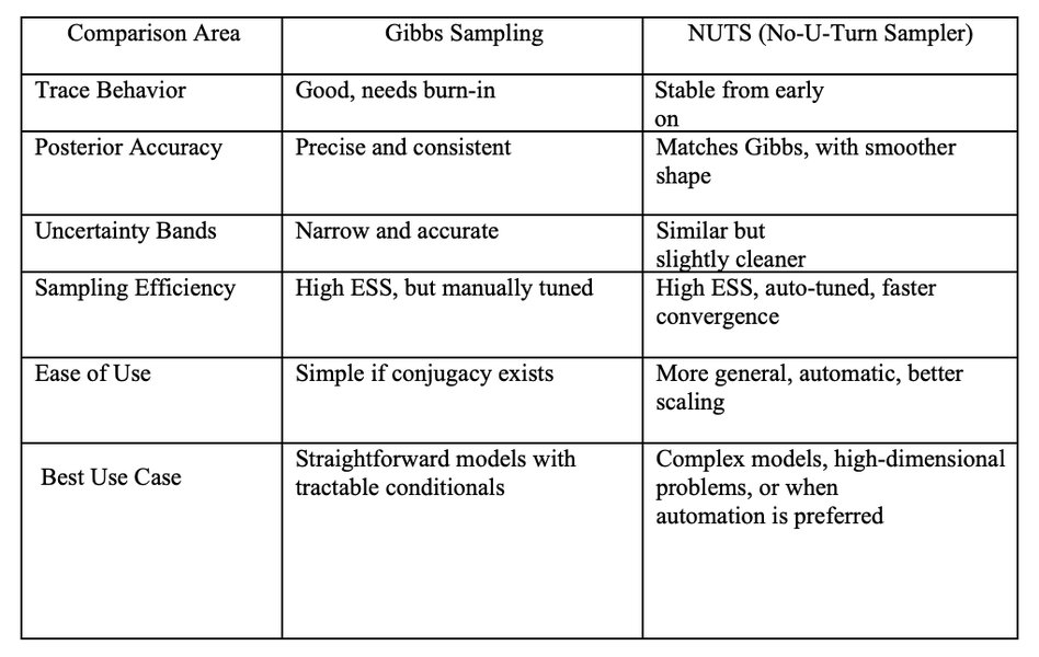
To summarize the distinctions and relationships between these powerful simulation methods, the following table outlines their primary attributes and applications.
| Feature | Monte Carlo Simulation | Gibbs Sampling | Metropolis-Hastings Algorithm |
|---|---|---|---|
| Origin/History | Manhattan Project (1940s), Ulam & von Neumann | Popularized in Bayesian statistics (early 1990s), named after J.W. Gibbs | Metropolis et al. (1953), generalized by Hastings (1970) |
| Core Concept | Repeated random sampling to obtain numerical results for complex problems with uncertainty. | Iterative sampling from full conditional distributions of each variable, given all others. | Proposes new states and accepts/rejects them based on an acceptance probability, handles unnormalized target distributions. |
| Relationship | Broad framework for probabilistic simulation. | A special case of MCMC, often a special case of Metropolis-Hastings (acceptance probability typically 1). | General MCMC method; Gibbs sampling is a specialized form of MH. |
| Strengths | Versatile, good for optimization, numerical integration, risk assessment. | Efficient for high-dimensional problems where conditionals are known; fast mixing if applicable. | Highly flexible, can sample from any distribution where density is known (up to a constant); handles complex geometries. |
| Limitations | Can be computationally intensive for high-precision results; may not efficiently explore complex distributions. | Requires easily samplable full conditional distributions; can struggle if conditionals are complex or unknown. | Choice of proposal distribution is critical for efficiency; can suffer from slow mixing or high rejection rates if poorly chosen. |
| Typical Applications | Finance, project management, engineering, healthcare modeling. | Bayesian inference, latent variable models (e.g., LDA), image analysis, genomics. | General Bayesian inference, statistical physics, machine learning models with complex posterior distributions. |
Frequently Asked Questions
What is the main difference between Monte Carlo and MCMC methods?
When would I choose Gibbs sampling over Metropolis-Hastings?
What does "burn-in" mean in the context of MCMC?
Is it possible to combine Gibbs sampling and Metropolis-Hastings?
Why is the normalization constant important for direct sampling but not for Metropolis-Hastings?
Conclusion
Monte Carlo simulation, Gibbs sampling, and the Metropolis-Hastings algorithm represent a cornerstone of modern computational science. From their wartime origins in nuclear physics to their widespread application across finance, engineering, machine learning, and biology, these methods have continuously evolved to tackle increasingly complex probabilistic challenges. Monte Carlo provides the foundational approach of using random sampling; Metropolis-Hastings offers a general framework for exploring distributions even without full analytical tractability; and Gibbs sampling provides a highly efficient, specialized alternative when conditional distributions are accessible. Together, they empower researchers and practitioners to quantify uncertainty, estimate intractable parameters, and gain profound insights into complex systems where deterministic solutions fall short.
Recommended Further Exploration
- How do MCMC methods enhance Bayesian inference?
- What are the best practices for tuning proposal distributions in Metropolis-Hastings?
- How can I assess the convergence of my MCMC simulations?
- What are the cutting-edge applications of Monte Carlo methods in quantitative finance?