

Key Insights into Naïve Bayes
- Foundation in Bayes' Theorem: Naïve Bayes is a probabilistic classification algorithm built upon Bayes' Theorem, leveraging prior knowledge and likelihoods to determine posterior probabilities for classification.
- The "Naïve" Assumption: Despite its name, the algorithm simplifies calculations by assuming features are conditionally independent given the class label. This assumption, while often violated in reality, leads to remarkable efficiency and performance.
- Text Classification Champion: Naïve Bayes excels in text-based tasks like spam detection, sentiment analysis, and document categorization due to its ability to handle high-dimensional and sparse data efficiently.
Introduction to Naïve Bayes: A Probabilistic Paradigm
Naïve Bayes stands as a foundational yet remarkably effective supervised learning algorithm within the realm of machine learning. It is primarily employed for classification tasks, where the objective is to assign an input data point to one of several predefined categories based on its inherent features. What sets Naïve Bayes apart is its deeply rooted probabilistic nature, drawing its theoretical strength directly from Bayes' Theorem.
This algorithm is particularly renowned for its efficiency and simplicity, making it a go-to choice for scenarios involving large datasets and high-dimensional feature spaces, such as those commonly encountered in text analysis. The "naïve" moniker, often a point of curiosity, refers to a crucial simplifying assumption: that all features used in the classification process are conditionally independent of one another, given the class variable. While this assumption rarely holds perfectly true in complex real-world data, the algorithm's performance in practice, especially in fields like text classification, is surprisingly robust.
Naïve Bayes is a set of supervised learning algorithms based on applying Bayes' Theorem with the assumption of conditional independence between features. Its utility spans various domains, from the mundane task of sifting spam emails from legitimate ones to the more nuanced challenge of discerning sentiment in customer reviews.
Decoding the Core: Bayes' Theorem and the Naïve Assumption
At the heart of the Naïve Bayes classifier lies Bayes' Theorem, a fundamental principle of probability theory that describes how to update the probability of a hypothesis as more evidence or information becomes available. For classification, this theorem provides a framework to calculate the probability of a data point belonging to a particular class, given the observed features.
Bayes' Theorem Unpacked
The mathematical formulation of Bayes' Theorem is expressed as:
\[P(y|X) = \frac{P(X|y) \cdot P(y)}{P(X)}\]Let's break down each component:
- \(P(y|X)\): This is the posterior probability, representing the probability of the class \(y\) (e.g., "spam" or "not spam") given the observed features \(X = (x_1, x_2, ..., x_n)\). This is what the algorithm aims to predict.
- \(P(X|y)\): This is the likelihood, which is the probability of observing the features \(X\) given that the class is \(y\).
- \(P(y)\): This is the prior probability of the class \(y\), representing the initial probability of a class before considering any features from the current data point. It's simply the frequency of that class in the training data.
- \(P(X)\): This is the evidence or normalizing constant, representing the probability of observing the features \(X\). Since \(P(X)\) remains constant across all classes for a given input, it can be disregarded during the class comparison phase, simplifying the calculation to a proportionality: \(P(y|X) \propto P(X|y) P(y)\).
The "Naïve" Independence Assumption
The pivotal simplification that gives Naïve Bayes its name is the assumption of conditional independence of features. This means that given the class label, the presence or absence of one feature does not affect the presence or absence of any other feature. Mathematically, this transforms the likelihood term \(P(X|y)\) from a complex joint probability into a simple product of individual conditional probabilities:
\[P(X|y) = \prod_{i=1}^{n} P(x_i | y)\]Where \(x_i\) represents an individual feature. This radical simplification drastically reduces the computational complexity of the model, allowing it to be trained and make predictions very quickly, even with a massive number of features. Despite the fact that this independence assumption is rarely perfectly met in real-world datasets (e.g., in text, words are often contextually dependent), Naïve Bayes frequently delivers surprisingly competitive performance.
The algorithm then computes this modified posterior probability for each possible class and selects the class with the highest probability as its prediction. This efficiency, combined with its interpretability, makes it a powerful tool, particularly in domains like natural language processing.
Operationalizing Naïve Bayes: A Step-by-Step Guide
The working mechanism of the Naïve Bayes algorithm can be broken down into a series of clear steps, which illustrate how it processes data to make classifications.
-
Calculating Prior Probabilities \(P(y)\)
The first step involves determining the prior probability for each class. This is simply the frequency of each class in the training dataset. For example, if a training set has 100 emails, and 20 of them are spam, then \(P(\text{spam}) = 20/100 = 0.2\).
-
Estimating Likelihoods \(P(x_i | y)\)
Next, the algorithm calculates the likelihood of each feature \(x_i\) given each class \(y\). This involves counting how often a specific feature appears within instances of a particular class. For continuous features, a distribution (like Gaussian) might be assumed. For categorical or discrete features (common in text), these are typically estimated using frequency counts. For instance, to classify spam, you might calculate \(P(\text{"free"} | \text{spam})\), which is the number of times "free" appears in spam emails divided by the total number of words in spam emails.
-
Computing Posterior Probability for New Data
When a new, unseen data point (e.g., an email) needs to be classified, the algorithm uses the calculated priors and likelihoods to compute the posterior probability for each class. Using the simplified formula derived from the independence assumption, it multiplies the prior probability of each class by the likelihoods of all the features present in the new data point, conditioned on that class:
\[P(y|X) \propto P(y) \prod_{i=1}^{n} P(x_i | y)\] -
Predicting the Class
Finally, the algorithm compares the posterior probabilities calculated for all possible classes. The class with the highest posterior probability is then assigned as the predicted label for the new data point.
This process highlights the algorithm's computational efficiency, as it primarily involves counting frequencies and simple multiplications, making it suitable for large-scale datasets.
Variants of Naïve Bayes for Diverse Data
While the fundamental principles remain consistent, Naïve Bayes classifiers come in several variants, each tailored to different types of data distributions and feature characteristics. Understanding these variants is crucial for selecting the most appropriate model for a given task.
-
Multinomial Naïve Bayes (MultinomialNB)
This variant is arguably the most popular for text classification. It is specifically designed for features that represent counts or frequencies, such as word counts in a document (the "bag-of-words" model) or term frequency-inverse document frequency (TF-IDF) vectors. It assumes that features follow a multinomial distribution, meaning it's well-suited for discrete data representing the number of times an event (like a word appearing) has occurred.
-
Bernoulli Naïve Bayes (BernoulliNB)
Unlike Multinomial Naïve Bayes, Bernoulli Naïve Bayes is used when features are binary, indicating the presence or absence of a particular characteristic. In text classification, this would mean simply noting whether a word appears in a document (1) or not (0), rather than counting its occurrences. It's effective for document classification where the presence of a keyword is more indicative than its frequency.
-
Gaussian Naïve Bayes
This variant is applied when the features are continuous numerical values. It assumes that these continuous features for each class are distributed according to a Gaussian (normal) distribution. For each feature and class, the algorithm estimates the mean and variance from the training data, which are then used to calculate the likelihood \(P(x_i | y)\) using the probability density function of the Gaussian distribution.
-
Complement Naïve Bayes (ComplementNB)
An adaptation of Multinomial Naïve Bayes, Complement Naïve Bayes is particularly useful for imbalanced datasets, where some classes have significantly fewer training examples than others. It computes model weights using statistics from the complement of each class (i.e., all samples not belonging to that class), which can help to mitigate the bias towards majority classes.
The Power of Naïve Bayes in Text Classification
Naïve Bayes has carved out a significant niche in the domain of Natural Language Processing (NLP), particularly excelling in various text classification tasks. Its inherent simplicity, computational efficiency, and robust performance, even with the "naïve" assumption, make it a preferred choice for many real-world applications dealing with textual data.
In text classification, documents are typically represented using a "bag-of-words" model, where the order and grammar of words are disregarded, but their frequency or presence is noted. Each unique word in the vocabulary often becomes a feature, leading to very high-dimensional data, which Naïve Bayes handles efficiently.
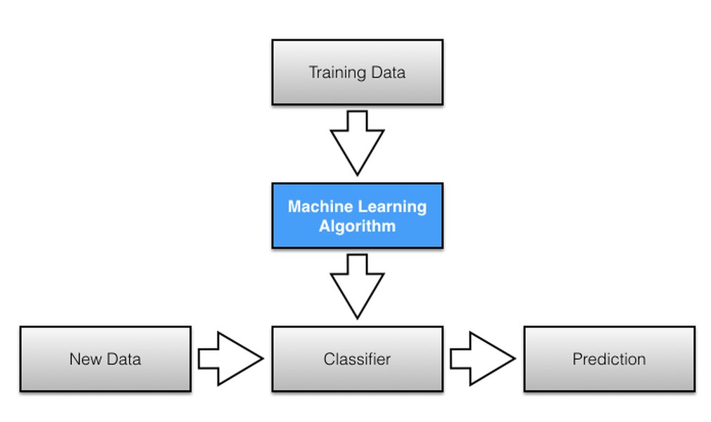
A conceptual illustration of the Naïve Bayes learning algorithm applied to text classification.
Key Applications of Naïve Bayes in Text
-
Spam Detection
One of the most classic and widely successful applications of Naïve Bayes is filtering spam emails. The algorithm learns from a corpus of labeled emails (spam or not spam) to identify patterns of words associated with each category. For an incoming email, it calculates the probability that the email is spam given the words it contains, and classifies it accordingly. Words like "free," "offer," "urgent," or specific combinations often strongly correlate with spam, which Naïve Bayes effectively leverages.
-
Sentiment Analysis
Naïve Bayes is frequently used to determine the emotional tone or sentiment expressed in a piece of text (e.g., product reviews, social media posts). By analyzing words and phrases, it can classify text as positive, negative, or neutral. For example, words like "amazing," "excellent," "love" might indicate positive sentiment, while "terrible," "hate," "disappointed" suggest negative sentiment. The algorithm learns these associations from training data.
-
Document Categorization/News Classification
This involves assigning entire documents or articles to predefined topics or categories (e.g., sports, politics, technology, finance). Naïve Bayes examines the word distribution within a document and compares it to the word distributions observed in documents from various categories during training. A document with words like "economy," "stocks," and "inflation" is likely to be classified under "finance."
-
Language Detection
Naïve Bayes can be trained to identify the language of a given text snippet by analyzing the frequency of characters or short sequences of characters (n-grams) unique to different languages.
The speed and simplicity of Naïve Bayes make it suitable for real-time text processing applications, such as live chat moderation or instant message filtering. Its ability to perform well even with relatively small training datasets and its robustness to irrelevant features further cement its position as a go-to algorithm for text classification.
Illustrative Examples: Naïve Bayes in Action
To solidify the understanding of Naïve Bayes, let's explore detailed examples, focusing on its most prominent application: text classification. These examples demonstrate how the theoretical framework translates into practical prediction.
Example 1: Spam Email Classification
Imagine a simplified email spam filter. Our goal is to classify an incoming email as either "spam" or "not spam" based on the words it contains. For this example, let's consider a new email with the words "dear" and "friend".
Training Data Insights (Hypothetical):
- Total emails: 10
- Spam emails: 4 (e.g., "dear friend, win free money", "earn money now", "free offer", "friend get free")
- Not Spam emails: 6 (e.g., "dear team, meeting tomorrow", "project update", "hello friend", "daily news", "work schedule", "important document")
Step-by-step calculation for an email with "dear" and "friend":
-
Calculate Prior Probabilities:
- \(P(\text{Spam}) = 4/10 = 0.4\)
- \(P(\text{Not Spam}) = 6/10 = 0.6\)
-
Calculate Likelihoods (using add-one smoothing to avoid zero probability):
Assume vocabulary size \(V\) for simplicity (e.g., 10 unique words in total across all training emails). The formula for likelihood with smoothing is \((count(\text{word in class}) + 1) / (count(\text{total words in class}) + V)\).
- For "dear" in Spam: (Count of "dear" in Spam + 1) / (Total words in Spam emails + V)
- For "friend" in Spam: (Count of "friend" in Spam + 1) / (Total words in Spam emails + V)
- And similarly for "Not Spam".
- \(P(\text{dear}|\text{Spam}) = 0.1\)
- \(P(\text{friend}|\text{Spam}) = 0.15\)
- \(P(\text{dear}|\text{Not Spam}) = 0.2\)
- \(P(\text{friend}|\text{Not Spam}) = 0.25\)
Let's use simplified hypothetical likelihoods after smoothing for demonstration:
-
Compute Posterior Probability (Numerator only):
- \(P(\text{Spam}|\text{dear, friend}) \propto P(\text{Spam}) \cdot P(\text{dear}|\text{Spam}) \cdot P(\text{friend}|\text{Spam})\)
- \(P(\text{Spam}|\text{dear, friend}) \propto 0.4 \cdot 0.1 \cdot 0.15 = 0.006\)
- \(P(\text{Not Spam}|\text{dear, friend}) \propto P(\text{Not Spam}) \cdot P(\text{dear}|\text{Not Spam}) \cdot P(\text{friend}|\text{Not Spam})\)
- \(P(\text{Not Spam}|\text{dear, friend}) \propto 0.6 \cdot 0.2 \cdot 0.25 = 0.030\)
-
Predict Class:
Since \(0.030 > 0.006\), the email containing "dear" and "friend" would be classified as "Not Spam".
This example demonstrates how the simple multiplication of probabilities, thanks to the independence assumption, allows Naïve Bayes to efficiently classify text.
Example 2: News Article Categorization
Consider classifying a news article into "Sports" or "Politics". A new article contains the words "team" and "vote".
Hypothetical Training Data Analysis:
- Articles classified as "Sports" frequently contain "team", "goal", "player".
- Articles classified as "Politics" frequently contain "vote", "government", "election".
Applying Naïve Bayes:
The algorithm would calculate:
- \(P(\text{Sports}|\text{article with 'team', 'vote'}) \propto P(\text{Sports}) \cdot P(\text{team}|\text{Sports}) \cdot P(\text{vote}|\text{Sports})\)
- \(P(\text{Politics}|\text{article with 'team', 'vote'}) \propto P(\text{Politics}) \cdot P(\text{team}|\text{Politics}) \cdot P(\text{vote}|\text{Politics})\)
By comparing these two values, the article would be assigned to the category with the higher probability. Even if "team" appears in a politics article (e.g., "political team"), the combination of probabilities would likely favor "Politics" if "vote" is a strong indicator for that category.
Evaluating Naïve Bayes: Strengths and Challenges
Like any algorithm, Naïve Bayes possesses a distinct set of advantages that make it suitable for specific tasks, alongside limitations that necessitate careful consideration during implementation.
Advantages of Naïve Bayes
-
Simplicity and Speed
Naïve Bayes is remarkably simple to understand and implement. Its training process is exceptionally fast, primarily involving counting frequencies and performing basic arithmetic operations. This makes it ideal for real-time predictions and applications where computational resources are a constraint.
-
Efficiency with High-Dimensional Data
It performs exceptionally well with datasets that have a large number of features, which is characteristic of text data (e.g., thousands of unique words). The conditional independence assumption simplifies computations to a point where even high-dimensionality doesn't lead to significant performance bottlenecks.
-
Requires Less Training Data
Compared to more complex models, Naïve Bayes can perform effectively even with a relatively small amount of training data to estimate the necessary parameters (priors and likelihoods). It also tends to generalize well from limited samples.
-
Probabilistic Output
The algorithm provides a probabilistic output (the posterior probability), which can be useful for ranking predictions or when a measure of confidence in the classification is required, not just a binary label.
-
Robust to Irrelevant Features
While sensitive to correlated features, Naïve Bayes can be quite robust to the presence of irrelevant features, especially in text classification, as these features will simply have low likelihoods and won't significantly influence the final probability.
Limitations of Naïve Bayes
-
Strong Independence Assumption
The most significant limitation is its "naïve" assumption that all features are conditionally independent given the class. In reality, features are often highly correlated (e.g., in text, the word "New" is often followed by "York"). When this assumption is severely violated, the algorithm's performance can degrade, and its probability estimates might be overconfident.
-
Zero Probability Problem
If a particular feature value (e.g., a word) does not appear with a certain class in the training data, the likelihood \(P(x_i|y)\) for that feature will be zero. Due to the multiplicative nature of the formula, this zero will propagate, causing the entire posterior probability for that class to become zero, regardless of other features. This issue is typically handled using smoothing techniques (e.g., Laplace smoothing or add-one smoothing), which add a small "pseudo-count" to avoid zero probabilities.
-
Sensitivity to Feature Representation
The performance of Naïve Bayes can be sensitive to how features are represented, particularly whether they are categorical, binary, or continuous, and which variant of the algorithm (Multinomial, Bernoulli, Gaussian) is chosen.
Despite these limitations, Naïve Bayes often serves as an excellent baseline model due to its simplicity and efficiency, frequently outperforming more complex algorithms in specific domains like text classification.
Delving Deeper: Visualizing Naïve Bayes Concepts
To further enhance understanding, a mindmap provides a structured overview of the key concepts and relationships associated with Naïve Bayes, bringing together the theoretical underpinnings and practical applications discussed.
This mindmap visually organizes the various components of Naïve Bayes, from its theoretical foundation in Bayes' Theorem and the critical "naïve" assumption, through its operational steps and different variants. It also comprehensively outlines its wide range of applications, particularly in text classification, as well as its notable advantages and inherent limitations. This structured view helps in grasping the interconnections between different aspects of the algorithm.
Visualizing Naïve Bayes for Text Classification
The video, "Naive Bayes: Text Classification Example," provides an excellent visual and practical walkthrough of how the Naïve Bayes algorithm operates specifically within the context of text classification. It demystifies the concepts by using a tangible example, making the theoretical aspects of Bayes' Theorem and the independence assumption much easier to grasp. The video likely illustrates how to calculate prior probabilities and likelihoods from a sample dataset and then applies these to classify a new text instance. This visual aid is incredibly relevant because text classification is the primary domain where Naïve Bayes truly shines, and seeing the step-by-step application reinforces the learned concepts, particularly how word frequencies and their probabilities contribute to the final classification decision.
Comparative Overview: Naïve Bayes Characteristics
The table below summarizes key characteristics and considerations for Naïve Bayes, offering a quick reference for its attributes and typical use cases.
| Characteristic | Description | Impact/Relevance |
|---|---|---|
| Algorithm Type | Supervised Learning, Probabilistic Classifier | Learns from labeled data, outputs probabilities for class predictions. |
| Core Principle | Bayes' Theorem | Calculates the probability of a class given features based on prior knowledge. |
| Key Assumption | Conditional Independence of Features | Simplifies calculations, allows for efficient processing of high-dimensional data. |
| Data Types Supported | Categorical, Binary (Bernoulli), Continuous (Gaussian), Count-based (Multinomial) | Versatility across different feature types. |
| Primary Use Cases | Text Classification (Spam Filter, Sentiment Analysis, Document Categorization) | Highly effective due to efficiency with sparse, high-dimensional text data. |
| Training Speed | Very Fast | Simple frequency counting and multiplication operations. |
| Prediction Speed | Very Fast | Minimal computation required for new instances. |
| Memory Footprint | Low | Stores only counts and probabilities. |
| Robustness to Irrelevant Features | Good | Features with low likelihoods have minimal impact. |
| Handling of Missing Values | Requires imputation or special handling; not inherently robust. | Missing data needs preprocessing, as it cannot contribute to likelihood calculations. |
This table systematically outlines the fundamental characteristics of Naïve Bayes, reinforcing its strengths as a fast, simple, and effective probabilistic classifier, especially for text-related tasks. It also subtly hints at areas where preprocessing or specific model variants might be necessary.
Frequently Asked Questions (FAQ) about Naïve Bayes
What does "Naïve" mean in Naïve Bayes?
Why is Naïve Bayes particularly useful for text classification?
What is the "zero probability problem" in Naïve Bayes, and how is it addressed?
What are the different types of Naïve Bayes classifiers?
- Multinomial Naïve Bayes: Best for discrete features like word counts in text.
- Bernoulli Naïve Bayes: Used for binary features, indicating presence or absence (e.g., a word is either in a document or not).
- Gaussian Naïve Bayes: Applies to continuous features, assuming they follow a Gaussian (normal) distribution.
Conclusion
Chapter 40, "Naïve Bayes: Probabilistic Classification," provides a comprehensive understanding of a powerful yet simple algorithm that remains a cornerstone in supervised learning, especially for text classification. Rooted in Bayes' Theorem, its strength lies in its "naïve" assumption of feature independence, which dramatically simplifies computations, allowing for efficient processing of high-dimensional datasets. While its core assumption is often violated in real-world scenarios, Naïve Bayes consistently delivers competitive performance in tasks such as spam detection, sentiment analysis, and document categorization. Its advantages in terms of speed, simplicity, and low data requirements make it an indispensable tool for data scientists and a foundational concept for anyone delving into machine learning. Understanding its mechanics, variants, and practical applications, along with its limitations and the common solutions (like smoothing), equips learners with a robust probabilistic classification method that serves both as a strong baseline and a practical solution for a wide array of problems.
Recommended Further Exploration
- How does Laplace smoothing impact Naive Bayes performance?
- Comparing Naive Bayes with other classification algorithms like SVM and Logistic Regression
- Advanced text preprocessing techniques for Naive Bayes classifiers
- Real-world case studies of Naive Bayes in spam filtering