Illustrating Dynamic Change in Neural Populations

Exploring how neurons interact and exhibit emergent behavior

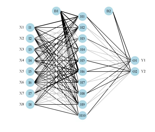
Key Highlights

Computational and Analytical Frameworks: Use mathematical models and computational simulations to reveal the dynamic evolution of neural activity.
Visualization Techniques: Employ dimensionality reduction, state-space analyses, and data visualization tools to observe complex interactions.
Experimental and Theoretical Approaches: Integrate neuroimaging, electrophysiology, and experimental manipulations to validate models and demonstrate emergent properties.

Understanding Neural Population Dynamics

Theoretical Background

Neural population dynamics refer to the collective behavior of groups of neurons that interact over time to produce complex brain functions. Instead of focusing on individual neurons, this approach studies the evolution of their collective states, often described using dynamical systems theory. In these systems, each neuron’s activity is influenced by its own properties as well as by its interactions with other neurons, which can be captured through mathematical models and simulations.

Emergent properties arise when the neural population exhibits behaviors or functions that are not inherent in the individual components. These can include rhythmic oscillations, synchronization, pattern formation, and even higher cognitive functions. The challenge is to bridge the understanding between microscopic activities (i.e., the firing patterns of individual neurons) and macroscopic phenomena (i.e., cognitive and behavioral outputs).

Computational Modeling and Analytical Techniques

Dynamic Population Models

A major step in illustrating dynamic changes is the development and use of mathematical models that simulate neural population dynamics. Models such as linear dynamic models and recurrent neural networks (RNNs) capture how neuronal firing rates evolve over time. These simulations help in predicting how slight modifications in parameters (e.g., synaptic strength or connectivity patterns) can lead to vastly different outcomes, thereby revealing the basis of emergent properties.

For example, by using tools like principal component analysis (PCA) or t-distributed Stochastic Neighbor Embedding (t-SNE), you can reduce the dimensionality of complex neural recordings. This reduction makes it possible to visualize patterns and trajectories in a low-dimensional space. In these representations, trajectories may converge or diverge, switching between different states that embody sensory processing, decision-making, or motor actions.

State-Space Analysis and Dynamical Systems

State-space analysis allows researchers to track the evolution of neural population states. In these analyses, neural activity is plotted in a multidimensional space where each axis may represent the activity of a neural subpopulation. The trajectories that these populations follow offer insights into how external stimuli or internal regulatory mechanisms drive changes over time.

A common demonstration involves plotting the state-space trajectories of a neural circuit during tasks such as working memory or motor planning. Such plots capture how neurons transition between different states, with emergent properties like rhythmicity or periodicity emerging naturally from the population dynamics. By systematically altering the initial conditions in these models, you can uncover the conditions that are critical for the emergence of these properties.

Emergent Behavior Inference Techniques

Techniques like Emergent Property Inference (EPI) are particularly useful when modeling the behavior of neural circuits. EPI involves varying model parameters to observe the conditions under which a particular emergent property (such as oscillations or synchronization) prominently appears. Plotting the parameter distributions alongside the observed emergent behavior provides a clear illustration of how multiple parameterizations can lead to the same state.

Visualization Approaches for Neural Dynamics

Data Visualization and Dimensionality Reduction

Visualization is one of the most compelling ways to illustrate dynamic changes in neural population activity. High-dimensional neural data is often condensed using dimensionality reduction techniques like PCA or t-SNE. These methods help reveal patterns that are otherwise obscured when examining raw data.

Creating time-series plots, heatmaps, or scatter plots can effectively showcase the evolution of neural activity. Heatmaps, for instance, can be used to display the firing rates of neurons across time frames. As neural population activity is recorded, these heatmaps can be animated to visually demonstrate how synchronization, de-synchronization, or oscillations occur over a specific period.

Simulative Visual Representations

Using computational tools, one can simulate neural dynamics in virtual neural circuits. Visual outputs from these simulations, such as videos or animated graphs, can show how trajectories in neural state-space evolve over time. Consider a simulation of a neural circuit like the stomatogastric ganglion (STG) that generates rhythmic patterns for digestion.

By plotting the activity trajectories in a state-space, you can highlight how different initial conditions or network perturbations lead to a convergence towards steady rhythmic activity. This emergent rhythm is a clear example of how the collective activity of multiple neurons gives rise to a coherent function that is not inherent in any single neuron.

Experimental Techniques for Illustration

While modeling and computational simulations provide substantial insights, experimental techniques are crucial to validate these models. Neuroimaging techniques such as functional magnetic resonance imaging (fMRI), optical imaging, and electrophysiology can capture real-time neural activity.

By recording neural population activity during specific tasks, researchers can correlate observed patterns with those predicted by models. Techniques like optogenetics also allow for the manipulation of neural activity. For instance, activating or inhibiting certain neural populations can demonstrate in a controlled setting how these populations transition between states and give rise to emergent properties.

Integrating Computational Models with Empirical Data

Case Study: Rhythmic Neural Activity

One practical example of illustrating neural population dynamics involves studying rhythmic patterns in neural circuits. Consider a neural circuit that generates a rhythmic output, such as the patterns needed for locomotion or the cyclical activation seen in breathing. Computational models of these circuits can be simulated using dynamical systems theory.

Using techniques such as state-space analysis, you can depict how distinct trajectories converge to generate a stable oscillatory output. In these cases, emergent properties like periodic oscillations are not explicitly programmed but naturally arise from the interactions between neurons with varying degrees of excitability and connectivity.

The approach typically involves:

Model Setup: Define the neural circuit with parameters that assign specific roles to different types of neurons.
Parameter Variation: Systematically vary synaptic strengths or connectivity patterns and monitor changes in the network behavior.
State-Space Plotting: Project the neural dynamics into a lower-dimensional state space using PCA, and plot the trajectories.
Emergent Pattern Visualization: Highlight how despite different starting conditions, trajectories converge into stable rhythmic or oscillatory regimes.

This process clearly shows how neural populations collectively exhibit emergent properties that are critical for functioning in biological systems.

Visualization Tools and Software

A number of visualization tools and software packages can aid in illustrating neural dynamics. MATLAB, Python (with libraries such as NumPy, SciPy, and Matplotlib), and specialized simulation environments like NEURON or Brian are frequently used for this purpose. These tools allow one to build simulations, run data analyses, and generate insightful visualizations in the form of plots, animations, or interactive dashboards.

Below is a table summarizing common tools and their applications:

Tool/Software	Application	Key Feature
MATLAB	Simulation and Data Analysis	Robust computational environment and visualization capabilities.
Python (NumPy, SciPy, Matplotlib)	Modeling and Plotting	Open-source libraries for simulation, analysis, and interactive plots.
NEURON	Neural Simulation	Specialized environment for modeling neural circuits with high fidelity.
Brian	Spiking Neural Networks	Efficient simulation of spiking neurons and population dynamics.

Bridging Theory and Practice: Experimental Illustrations

Laboratory Techniques

Experimental data not only reinforces computational models but also provides a means to validate emergent behaviors observed in simulations. Electrophysiological recordings can capture the firing patterns of neurons at high temporal resolutions, thereby revealing the rapid dynamic changes of neural populations. These recordings, when processed through state-space analysis, can mimic and confirm the patterns predicted by computational practices.

In addition to electrophysiology, modern imaging techniques like fMRI or optical imaging capture the collective behavior of neurons on a larger scale. These techniques allow researchers to observe dynamic changes in brain regions, such as the prefrontal cortex during tasks, and link them to cognitive functions like working memory. By contrasting these empirical observations with theoretical models, one can create a comprehensive picture of neural population dynamics.

Combining Data and Simulations

A common strategy is to overlay simulation data with experimental data to highlight consistencies and discrepancies. Data visualization techniques, including animated heatmaps and dynamic network diagrams, vividly illustrate how neural interactions lead to emergent properties. These visualizations not only facilitate a deeper understanding for researchers but also make the underlying principles accessible to broader audiences.

Researchers often manipulate experimental conditions to observe changes in neural dynamics. For instance, altering synaptic strengths or interfering with connectivity using optogenetics allows one to observe a direct impact on the emergent behavior. When these changes are mirrored in computational models, it strengthens the validity of the theoretical framework.

Integrated Illustration Workflow and Practical Steps

Step-by-Step Workflow

The following outlines a practical workflow for illustrating dynamic changes in neural populations and their emergent properties:

Define the Neural Population: Identify the specific neural circuit or brain region of interest. Determine the key types of neurons and their connectivity.
Develop a Computational Model: Build a simulation employing dynamical systems theory. Choose appropriate mathematical models (e.g., differential equations or recurrent networks) to mimic the neural behavior.
Collect Experimental Data: Record neural activity using techniques like electrophysiology, fMRI, or optical imaging during relevant cognitive or motor tasks.
Apply Dimensionality Reduction: Process the high-dimensional neural data using PCA, t-SNE, or similar methods to visualize underlying neural trajectories.
Perform State-Space Analysis: Map the dynamic trajectories of the neural population, evaluating how different states emerge and evolve over time.
Visualize and Compare: Create visual representations (heatmaps, animated plots, and state-space diagrams) that overlay computational simulations with experimental data.
Interpret Emergent Phenomena: Evaluate how collective neural interactions result in emergent properties such as rhythmic oscillations, synchronization, or pattern formation.

Practical Example: Rhythmic Patterns in Neural Networks

To illustrate this process, consider a study focused on rhythmic activity within a neural circuit responsible for motor control. First, a computational model is created representing the circuit dynamics. Parameters such as synaptic strength, refractory periods, and connectivity patterns are included. Next, experimental data from electrophysiological recordings during a motor task is collected.

Using state-space analysis, trajectories of neural activity are plotted and compared with the output of the simulation. The observed rhythmic patterns in both data sets highlight how variations in initial conditions or network parameters eventually converge to produce consistent rhythmic outputs. This convergence demonstrates that while individual neurons may behave erratically, their collective interaction inevitably leads to emergent patterns that govern coherent motor functions.