Exploring Principal Component Analysis and Color Space Transformations

Highlights

Principal Component Analysis (PCA) is a powerful dimensionality reduction technique that linearly transforms data into a new coordinate system, ordered by variance.
Color Space Transformation involves converting color data between different color models, essential for accurate color representation and manipulation in digital imaging.
Both transformations are fundamental in various fields, including data analysis, image processing, and computer vision, for simplifying data, revealing underlying structures, and ensuring color fidelity.

Principal Component Analysis (PCA) and Color Space Transformation are two distinct yet valuable transformation techniques used across various disciplines, particularly in data analysis, image processing, and computer vision. While PCA focuses on reducing the dimensionality of complex datasets by identifying the directions of maximum variance, color space transformations are concerned with representing and manipulating color information in different mathematical models. This exploration delves into the principles, applications, and significance of both transformations, highlighting how they contribute to understanding data and visual information more effectively.

Principal Component Analysis (PCA): A Deep Dive into Dimensionality Reduction

Principal Component Analysis (PCA) is a widely used statistical method introduced by Karl Pearson in 1901. Its primary objective is to simplify high-dimensional datasets while retaining as much of the original variability as possible. This is achieved by transforming the data into a new set of coordinates, known as principal components, which are orthogonal (uncorrelated) and ordered according to the amount of variance they capture from the original data.

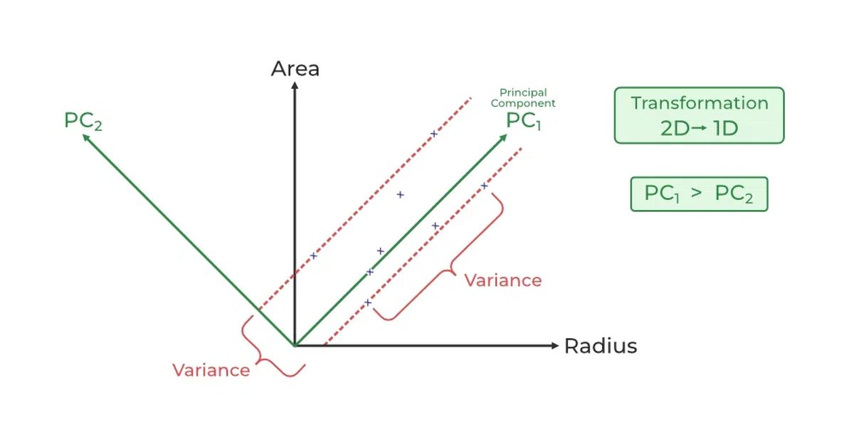
Conceptually, PCA can be understood as fitting a multi-dimensional ellipsoid to the data. The axes of this ellipsoid represent the principal components. The longest axis corresponds to the direction of the greatest variance, becoming the first principal component (PC1). Subsequent axes are orthogonal to the preceding ones and capture the remaining variance in descending order.

Illustration of PCA transformation showing the original axes and the new principal components.

Visualizing the transformation of data to principal components.

The Mathematical Foundation of PCA

At its core, PCA involves an orthogonal linear transformation. This transformation is derived from the eigenvectors and eigenvalues of the covariance matrix of the original data. The eigenvectors represent the directions of the principal components, and the corresponding eigenvalues indicate the magnitude of the variance along those directions.

Steps Involved in PCA:

Standardization: If variables have different units or scales, standardizing the data to have unit variance is often a crucial first step to prevent variables with larger scales from dominating the analysis. This involves subtracting the mean and dividing by the standard deviation for each variable.
Covariance Matrix Calculation: Compute the covariance matrix of the standardized data. This matrix summarizes the relationships and variances between the different variables.
Eigenvalue Decomposition: Calculate the eigenvalues and eigenvectors of the covariance matrix. The eigenvectors represent the principal components, and the eigenvalues indicate the amount of variance explained by each component.
Ordering Principal Components: Sort the eigenvectors in descending order based on their corresponding eigenvalues. The eigenvector with the highest eigenvalue is the first principal component, and so on.
Selecting Principal Components: Choose a subset of the principal components based on the amount of variance they capture. A common approach is to select components that collectively explain a significant percentage of the total variance (e.g., 95%).
Data Projection: Project the original data onto the selected principal components to obtain the reduced-dimensionality dataset. This is achieved by multiplying the original data (centered or standardized) by the transpose of the matrix formed by the selected eigenvectors.

The transformation can be represented mathematically. If \(X\) is the original data matrix and \(W\) is the matrix whose columns are the selected eigenvectors, the transformed data \(Y\) is given by:

\[ Y = XW \]

Where \(X\) is an \(n \times p\) matrix (n samples, p variables) and \(W\) is a \(p \times k\) matrix (p original variables, k selected principal components). The resulting transformed data \(Y\) is an \(n \times k\) matrix.

Mathematical representation of PCA showing data matrix and transformation matrix.

The mathematical basis of PCA involves matrix multiplication for data transformation.

Applications of PCA

PCA finds extensive applications in various fields:

Dimensionality Reduction: This is the most common application, especially in machine learning and data analysis, to handle datasets with a large number of features, reducing computational cost and mitigating the curse of dimensionality.
Noise Reduction: By discarding principal components with low variance (often associated with noise), PCA can help in denoising data.
Visualization: PCA can project high-dimensional data onto a 2D or 3D space (using the first two or three principal components) for easier visualization and identification of patterns or clusters.
Feature Extraction: The principal components can be considered as new features that are linear combinations of the original features, capturing the most important information.
Pattern Recognition: PCA is used in image recognition, facial recognition (eigenfaces), and other pattern recognition tasks.

While PCA is powerful for data reduction and revealing variance, it's important to note that it's a linear transformation and may not be optimal for datasets with non-linear structures. Also, the interpretability of the principal components can sometimes be challenging as they are combinations of the original variables.

Color Space Transformation: Navigating the Spectrum of Color

Color Space Transformation refers to the process of converting the numerical representation of a color from one color space to another. A color space is a mathematical model that describes how colors can be represented as a set of numerical values, typically three or four values representing color components.

Different color spaces are designed for various purposes, such as color display (RGB), printing (CMYK), or representing color in a way that is more perceptually uniform (like CIELAB or CIELUV). The need for color space transformation arises because different devices (cameras, monitors, printers) and applications use different color spaces, and accurate color reproduction or manipulation requires converting colors between these spaces.

Various color spaces offer different ways to represent color information.

Common Color Spaces and Their Transformations

Several color spaces are commonly used in digital imaging and graphics:

RGB (Red, Green, Blue):

This is an additive color model where colors are produced by combining different intensities of red, green, and blue light. It's widely used in displays and digital cameras. Different RGB color spaces exist, such as sRGB, Adobe RGB, and ProPhoto RGB, which have different gamuts (the range of colors they can represent).

CMYK (Cyan, Magenta, Yellow, Black):

This is a subtractive color model used in printing. Colors are created by subtracting varying amounts of cyan, magenta, yellow, and black ink from a white background.

HSV (Hue, Saturation, Value) / HSL (Hue, Saturation, Lightness):

These color spaces are often used for intuitive color selection and manipulation. Hue represents the pure color (like red, green, blue), saturation represents the color's intensity, and value or lightness represents its brightness.

CIELAB and CIELUV:

These are perceptually uniform color spaces designed to approximate human vision. In a perceptually uniform space, the same amount of change in numerical values corresponds to approximately the same amount of perceived color difference.

Mathematical Transformations Between Color Spaces

Color space transformations are typically achieved through mathematical formulas or matrix operations. These transformations map the color values from one space to another. The complexity of the transformation depends on the color spaces involved.

For example, the conversion between RGB and XYZ (a device-independent color space) often involves a linear transformation using a 3x3 matrix:

\[ \begin{pmatrix} X \ Y \ Z \end{pmatrix} = \begin{pmatrix} M_{11} & M_{12} & M_{13} \ M_{21} & M_{22} & M_{23} \ M_{31} & M_{32} & M_{33} \end{pmatrix} \begin{pmatrix} R \ G \ B \end{pmatrix} \]

Where \(M\) is the transformation matrix specific to the RGB color space being converted from. Conversions to or from perceptually uniform spaces like CIELAB often involve non-linear transformations.

Color space transformation is crucial for:

Color Management: Ensuring consistent color appearance across different devices.
Image Editing: Adjusting color balance, saturation, and hue.
Printing: Converting RGB images to CMYK for printing.
Computer Vision: Analyzing color properties of images for tasks like object detection and segmentation.

The accuracy of color space transformation is vital for maintaining color fidelity and achieving the desired visual output.

The Intersection of PCA and Color Spaces

While PCA and color space transformation are distinct, they can intersect, particularly in image processing tasks. Images, especially color images, are high-dimensional datasets. A color image in RGB space can be seen as three channels (Red, Green, Blue), each representing a dimension.

PCA can be applied to the pixel data of a color image to reduce its dimensionality or to analyze the principal variations in color. For instance, applying PCA to the RGB values of pixels across an image can reveal the main color patterns. This is sometimes referred to as "PCA color augmentation" or "Fancy PCA" in the context of data augmentation for machine learning, where the intensities of color channels are altered based on the principal components of the pixel colors.

PCA can be applied to color image data for analysis and processing.

Furthermore, PCA can be applied within different color spaces. Applying PCA to the data represented in a color space like HSV or CIELAB might yield different principal components than applying it to RGB data, as the correlation structure between the color components differs in each space. Studies have investigated the effect of applying PCA in different color spaces for tasks like face recognition, finding that the choice of color space can influence the performance of the PCA-based method.

Combining Transformations

In some image processing pipelines, both color space transformation and PCA might be used. For example, an image might first be converted to a color space like Lab (for its perceptual uniformity) before applying PCA for dimensionality reduction or feature extraction. This approach leverages the benefits of both techniques – the perceptually uniform representation from the color space transformation and the data reduction and variance prioritization from PCA.

Comparison and Complementarity

While both are transformations, their purposes and mechanisms are fundamentally different. The following table summarizes key distinctions:

Feature	Principal Component Analysis (PCA)	Color Space Transformation
Primary Goal	Dimensionality reduction, variance maximization, decorrelation	Changing the representation of color data, managing color appearance
Input Data	Multivariate data	Color data (typically 3 or 4 components)
Output Data	Transformed data in a new coordinate system with reduced dimensions (optional)	Color data in a different color space
Transformation Type	Linear (orthogonal)	Linear or non-linear, depending on the color spaces
Basis of Transformation	Eigenvectors of the covariance matrix	Mathematical formulas or matrices defined by the color space definitions
Applications	Data reduction, noise reduction, visualization, feature extraction, pattern recognition	Color management, image editing, printing, computer vision

Despite their differences, PCA and color space transformation can be complementary. Color space transformation can provide a more suitable representation of color data before applying PCA, potentially leading to more meaningful results in terms of identifying color variations or reducing redundancy.

Practical Considerations and Limitations

When applying PCA, it's important to consider the scale of the variables. As PCA is variance-focused, variables with larger scales can disproportionately influence the principal components. Standardizing the data can mitigate this. Additionally, PCA assumes linearity in the data structure; for non-linear relationships, other techniques might be more appropriate.

For color space transformations, the choice of color space depends heavily on the application. For instance, RGB is suitable for display, while CMYK is for print. Perceptually uniform spaces like CIELAB are preferred when the goal is to measure or manipulate color differences in a way that aligns with human perception. The accuracy of the transformation depends on the specific definitions of the color spaces and the implementation of the conversion formulas.

Color management workflows often involve a sequence of color space transformations to ensure color consistency from capturing an image to displaying or printing it. Understanding the characteristics and limitations of each color space and transformation is crucial for achieving accurate and predictable color results.

Conclusion

Principal Component Analysis and Color Space Transformation are powerful techniques with distinct roles. PCA excels at simplifying complex datasets by identifying and prioritizing directions of maximum variance, making it invaluable for dimensionality reduction and data analysis. Color Space Transformation is essential for accurately representing, manipulating, and reproducing color information across different devices and applications by converting between various color models.

While serving different primary purposes, these transformations can be used in conjunction, particularly in image processing, where color data is a key aspect. Applying PCA within specific color spaces or using color space transformation as a preprocessing step for PCA can enhance the analysis and processing of visual data. A solid understanding of both techniques is fundamental for effectively working with high-dimensional data and digital color information in numerous scientific and technical domains.

Frequently Asked Questions (FAQ)

What is the main difference between PCA and Color Space Transformation?

The main difference lies in their objectives. PCA is a dimensionality reduction technique that focuses on finding directions of maximum variance in a dataset, while Color Space Transformation is about converting color representations between different mathematical models to manage and reproduce colors accurately.

Can PCA be applied to color images?

Yes, PCA can be applied to color images. A color image can be treated as a multi-dimensional dataset (e.g., pixel values across RGB channels), and PCA can be used to reduce the dimensionality or analyze the principal variations in color information.

Why are there different color spaces?

Different color spaces exist because color needs to be represented and manipulated for various purposes and devices. Some spaces are device-dependent (like RGB for displays), while others are designed to be device-independent and perceptually uniform (like CIELAB), better representing how humans perceive color differences.

Is Color Space Transformation a linear transformation?

Color Space Transformation can be linear or non-linear depending on the color spaces involved. Conversions between some spaces, like RGB to XYZ, can be linear matrix multiplications, while conversions to perceptually uniform spaces like CIELAB often involve non-linear equations.

References

Last updated May 2, 2025