Interpreting Your Pearson Chi-Square Test Result: Decoding Significance

Key Insights from Your Chi-Square Result

Statistical Significance Threshold: A p-value of 0.064 is typically considered above the conventional significance level of 0.05. This suggests that the observed differences or associations are not statistically significant at this common threshold.
Implication for the Null Hypothesis: Since the p-value (0.064) is greater than 0.05, you would fail to reject the null hypothesis. This means there isn't sufficient evidence to conclude a statistically significant relationship or difference between the categorical variables being tested.
Chance vs. True Relationship: A p-value of 0.064 indicates that there is a 6.4% probability of observing the data (or more extreme data) if the null hypothesis were true. This is a relatively high probability, suggesting that the observed pattern could reasonably occur due to random chance.

The Pearson Chi-Square test is a fundamental statistical tool used to examine relationships between categorical variables. Your reported result, a p-value of 0.064, provides crucial information regarding the statistical significance of your findings. This comprehensive guide will delve into the intricacies of interpreting this specific p-value, explaining its implications for your null hypothesis, the role of significance levels, and the broader context of Chi-Square analysis.

Understanding the Pearson Chi-Square Test

The Pearson Chi-Square (χ²) test, often simply referred to as the Chi-Square test, is a non-parametric statistical test primarily applied to categorical data. Its core purpose is to determine whether there is a statistically significant difference between observed frequencies and expected frequencies in one or more categories of a contingency table. In essence, it assesses how likely it is that any observed differences or associations between sets of categorical data arose purely by chance.

There are two main types of Pearson's Chi-Square tests:

Chi-Square Test of Independence: This test evaluates whether two categorical variables are related or independent of each other. For example, it could be used to see if there's a relationship between a person's gender and their preferred learning medium.
Chi-Square Goodness-of-Fit Test: This test determines if an observed frequency distribution of a single categorical variable differs significantly from an expected frequency distribution. For instance, it could assess if a die is biased by comparing observed rolls to the expected equal distribution.

Both types utilize the same formula to calculate the chi-square test statistic (χ²), which quantifies the discrepancy between observed and expected counts. The calculation involves summing the squared differences between observed and expected values, divided by the expected values:

\[ \chi^2 = \sum \frac{(\text{O} - \text{E})^2}{\text{E}} \]

Where:

χ² is the Chi-Square test statistic.
O represents the observed frequency.
E represents the expected frequency.
∑ indicates the sum across all categories.

The expected frequencies are calculated based on the assumption that the null hypothesis is true (i.e., no relationship or no significant difference between observed and expected distributions). For a Chi-Square Test of Independence, the expected value for each cell in a contingency table is typically computed as: \(\frac{(\text{row total} \times \text{column total})}{\text{sample total}}\).

The Significance of the P-Value

The p-value is the cornerstone of interpreting Chi-Square test results. It represents the probability of obtaining a test statistic as extreme as, or more extreme than, the one calculated from your sample data, assuming that the null hypothesis is true. In simpler terms, it tells you the likelihood that your observed pattern occurred purely by random chance if there were no actual relationship or difference in the population.

Interpreting a P-Value of 0.064

Your p-value of 0.064 means there is a 6.4% chance of observing a difference or association as strong as, or stronger than, the one you found in your sample, if the variables are truly independent in the population (or if the observed distribution perfectly matches the expected distribution in a goodness-of-fit test). To make a decision, this p-value is compared against a predetermined significance level, often denoted as α (alpha).

The Conventional Significance Level (α = 0.05)

In most scientific and social science research, the widely accepted significance level (α) is 0.05. This means that researchers are willing to accept a 5% risk of incorrectly rejecting a true null hypothesis (a Type I error). The decision rule is straightforward:

If p-value ≤ α: Reject the null hypothesis. There is statistically significant evidence to conclude that an association or difference exists.
If p-value > α: Fail to reject the null hypothesis. There is not enough statistically significant evidence to conclude that an association or difference exists.

Applying the Rule to Your Result

Given your p-value of 0.064 and the conventional α = 0.05:

Since 0.064 > 0.05, you would fail to reject the null hypothesis. This implies that your data does not provide sufficient statistical evidence to conclude that there is a significant relationship or difference between the categorical variables you are testing. The observed differences could reasonably be attributed to random sampling variability.

Beyond the P-Value: Considering Context and Degrees of Freedom

While the p-value is critical, it's important to consider other factors for a complete interpretation. The Chi-Square test relies on "degrees of freedom" (df), which are essential for determining the p-value from the chi-square distribution. Degrees of freedom refer to the number of independent pieces of information used to calculate the statistic. For a Chi-Square Test of Independence with a contingency table of j rows and k columns, the degrees of freedom are calculated as \((j-1)(k-1)\).

Consider the following illustration of Chi-Square distribution curves at various degrees of freedom:

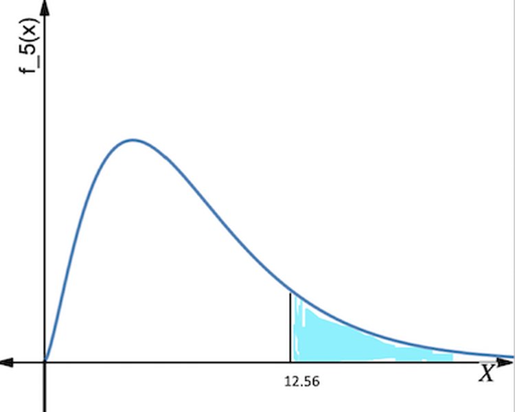
Figure 1: Examples of Chi-Square Distribution Curves for different degrees of freedom.

As the degrees of freedom increase, the chi-square distribution shifts to the right and becomes more symmetrical. The p-value is the area under this density curve to the right of your calculated chi-square test statistic.

The Chi-Square Statistic Itself

While the p-value is often the primary focus for significance, the Chi-Square statistic (χ²) itself measures the magnitude of the difference between observed and expected frequencies. A larger χ² value generally indicates a greater discrepancy, which, when coupled with a small p-value, suggests a statistically significant result. However, the χ² value doesn't have a direct "plain English" interpretation on its own; its meaning is tied to the degrees of freedom and the corresponding p-value.

Effect Size and Practical Significance

It's also important to distinguish between statistical significance and practical significance. A result can be statistically significant (p < 0.05) but have a very small effect size, meaning the relationship, while real, might not be practically important. Conversely, a result might not be statistically significant (like your 0.064 p-value) but hint at a potentially meaningful trend that warrants further investigation with a larger sample size or different study design. Measures like Cramer's V or Phi coefficient can be used to assess the strength of the association following a significant Chi-Square test.

Assumptions of the Chi-Square Test

For the Chi-Square test results to be valid, certain assumptions must be met:

Categorical Data: The variables must be categorical (nominal or ordinal).
Independence of Observations: Each observation must be independent of all other observations. This means that the outcome for one individual does not influence the outcome for another.
Expected Frequencies: The expected frequency in each cell of the contingency table should ideally be at least 5. If more than 20% of cells have expected counts less than 5, or any cell has an expected count less than 1, the Chi-Square approximation may not be accurate, and Fisher's Exact Test or Yates's correction might be more appropriate.
Random Sampling: The data should be collected from a random sample of the population.

Hypothesis Testing Framework with a P-Value of 0.064

Let's frame the interpretation of your 0.064 p-value within the standard hypothesis testing framework:

Formulating Hypotheses

Null Hypothesis (H₀): This hypothesis states that there is no association or difference between the categorical variables in the population. For example, if you're testing independence, H₀ would state that the two variables are independent.
Alternative Hypothesis (H₁ or H_a): This hypothesis states that there is an association or difference between the categorical variables in the population. It is the logical opposite of the null hypothesis.

With a p-value of 0.064 (which is > 0.05), you lack sufficient evidence to reject the null hypothesis. This means you cannot conclude that the alternative hypothesis is true. It does not prove the null hypothesis; it simply means your data does not provide strong enough evidence against it.

Illustrative Example of Chi-Square Interpretation

Imagine a study investigating whether there's an association between preferred news source (TV, Online, Print) and political affiliation (Democrat, Republican, Independent). After collecting data and performing a Chi-Square test, you obtain a p-value of 0.064.

Chi-Square Test Results: Preferred News Source vs. Political Affiliation
Statistic	Value	Degrees of Freedom (df)	Asymptotic Significance (p-value)
Pearson Chi-Square	4.567	2	0.064

In this hypothetical scenario, the p-value of 0.064 (assuming α = 0.05) suggests that there is no statistically significant association between preferred news source and political affiliation. The observed differences in preferences across political groups could be due to random chance.

Visualizing Statistical Outcomes: A Radar Chart Perspective

To further illustrate the concept of statistical significance and the decision-making process, let's use a radar chart. This chart will visually represent how different p-values compare against common significance thresholds and what their implications are for rejecting the null hypothesis. While your specific p-value is 0.064, this chart helps to contextualize it among other possible outcomes, providing a richer understanding of where your result stands.

Each axis on the radar chart will represent a key aspect of statistical decision-making, such as "Strength of Evidence Against Null," "Risk of Type I Error," and "Confidence in Rejecting Null." The data points will be opinionated analyses based on different p-value scenarios relative to a typical alpha of 0.05.

This radar chart visually depicts how a p-value of 0.064 positions itself relative to highly significant and clearly non-significant outcomes. Your result (P-value = 0.064) shows a moderate likelihood of chance occurrence and lower confidence in rejecting the null hypothesis compared to a highly significant result (P-value = 0.01). While not meeting the conventional 0.05 threshold, it's also not as high as a clearly non-significant p-value (e.g., 0.20), suggesting it's in a "gray area" where further investigation might be warranted.

The "Gray Area" of P-Values: What to Do with 0.064?

A p-value of 0.064 is very close to the conventional 0.05 significance level. This proximity often leads to discussions about its interpretation. While strictly speaking it's above the threshold, some researchers might consider it "marginally significant" or suggestive of a trend, especially if the sample size was small or the study is exploratory.

Acknowledge the Result: Clearly state the p-value and the chosen significance level in your report.
Fail to Reject H₀: Based on α = 0.05, you formally fail to reject the null hypothesis.
Discuss Implications: Explain that while not statistically significant at 0.05, the result is close and could warrant further research with a larger sample or a more refined experimental design.
Context is Key: Always interpret the statistical results within the context of your research question, existing literature, and the practical implications of your findings.

Beyond the P-Value: Exploring the "Why"

If your Chi-Square test yields a non-significant result like 0.064, it's beneficial to look deeper into the data, particularly at the observed versus expected counts. Examining which categories contributed most to the Chi-Square statistic can provide insights, even if the overall result isn't significant. Large differences between observed and expected counts in specific cells might indicate interesting patterns that just didn't reach statistical significance across the entire table. You can also visualize your data using bar charts, especially clustered or stacked bar charts, to compare subgroups within categories, which can provide a qualitative understanding of the relationships.

Using Statistical Software for Interpretation

Statistical software packages like SPSS, R, and Minitab automate the calculation and presentation of Chi-Square test results. They typically provide the Chi-Square statistic, degrees of freedom, and the p-value (often labeled as "Asymptotic Significance").

For instance, in SPSS, you would look at the "Pearson Chi-Square" row in the "Chi-Square Tests" table to find these values.

Video: A tutorial on how to run a Chi-Square test and interpret the output in SPSS.

This video demonstrates how to navigate SPSS to perform a Chi-Square test and highlights where to locate the key results, including the p-value, crucial for your interpretation. Understanding the software output ensures you correctly identify and utilize the relevant statistics for your conclusion.

Conclusion

A Pearson Chi-Square test result with a p-value of 0.064, when compared against a conventional significance level of 0.05, leads to the conclusion that you fail to reject the null hypothesis. This means there is not sufficient statistical evidence to claim a significant association or difference between your categorical variables at this chosen alpha level. While the result is not statistically significant, its proximity to the 0.05 threshold suggests that the observed pattern is not entirely random and might warrant further exploration or a larger study to definitively rule out or confirm a relationship. Always consider the context, assumptions of the test, and potential practical implications alongside the statistical p-value.

References

Last updated May 22, 2025