Unveiling the Nuances: Pearson vs. Spearman Correlation in Data Analysis

A comprehensive guide to understanding and applying two fundamental statistical measures of relationship.

Understanding the relationship between variables is a cornerstone of data analysis. While numerous statistical tools exist, Pearson's Product Moment Correlation and Spearman's Rank-Order Correlation stand out as two of the most widely used methods for quantifying the strength and direction of associations. Although both yield a coefficient ranging from -1 to +1, their underlying principles, assumptions, and suitability for different data types diverge significantly. Choosing the correct correlation method is crucial for accurate interpretation and valid conclusions.

Key Insights into Correlation Coefficients

Pearson's Correlation: Primarily assesses the strength and direction of a linear relationship between two continuous, normally distributed variables, sensitive to outliers.
Spearman's Correlation: Measures the strength and direction of a monotonic relationship (consistently increasing or decreasing, not necessarily linear) using ranked data, making it robust to outliers and suitable for ordinal or non-normally distributed continuous variables.
Choosing the Right Tool: The decision hinges on the nature of your data (continuous vs. ordinal), its distribution (normal vs. non-normal), and the type of relationship you hypothesize (linear vs. monotonic).

Pearson's Product Moment Correlation: The Linear Litmus Test

Pearson's Product Moment Correlation, often denoted as 'r', is a parametric statistical measure designed to quantify the strength and direction of a linear relationship between two continuous variables. It essentially evaluates how closely data points align with a straight line. The coefficient 'r' ranges from -1 to +1, where +1 signifies a perfect positive linear relationship (as one variable increases, the other increases proportionally), -1 indicates a perfect negative linear relationship (as one variable increases, the other decreases proportionally), and 0 suggests no linear relationship.

Core Principles and Assumptions

For Pearson's correlation to be appropriate, several assumptions must be met:

Linearity: The relationship between the two variables must be linear. A scatter plot can help visualize this.
Quantitative Variables: Both variables should be continuous, measured on an interval or ratio scale (e.g., age, income, height, temperature).
Normal Distribution: Both variables should be approximately normally distributed. Specifically, the data should follow a bivariate normal distribution.
Homoscedasticity: The variance of residuals should be constant across all levels of the independent variable.
No Significant Outliers: Pearson's 'r' is highly sensitive to outliers, which can significantly distort the correlation coefficient.

Calculating Pearson's 'r'

The Pearson correlation coefficient is calculated using the raw values of the variables, their respective means, and standard deviations. It represents the covariance of the two variables normalized by the product of their standard deviations. The formula for the sample Pearson correlation coefficient (r) is:

\[ r = \frac{\sum (x_i - \bar{x})(y_i - \bar{y})}{\sqrt{\sum (x_i - \bar{x})^2} \sqrt{\sum (y_i - \bar{y})^2}} \]

Where:

$ x_i $ and $ y_i $ are individual data points of variable X and Y, respectively.
$ \bar{x} $ and $ \bar{y} $ are the mean values of variable X and Y, respectively.

Illustrative Examples of Pearson's Use

Pearson's correlation is widely applied in various fields to quantify linear associations:

Positive Linear Relationship: Investigating the relationship between a person's age and income (as age increases, income tends to increase up to a certain point).
Negative Linear Relationship: Analyzing the relationship between the number of hours spent studying and the number of errors on a simple task (as study hours increase, errors might decrease).
Medical Field: Measuring the strength of the relationship between patient age and cholesterol levels, assuming a linear trend.
Manufacturing: Evaluating whether increases in temperature at a production facility are associated with decreasing thickness of a chocolate coating, if the relationship is expected to be linear.

Spearman's Rank-Order Correlation: Embracing Monotonicity

Spearman's Rank-Order Correlation, commonly denoted as 'ρ' (rho) or 'r_s', is a non-parametric statistical measure that assesses the strength and direction of a monotonic relationship between two variables. Unlike Pearson's, Spearman's does not require linearity or normal distribution. Instead, it converts the original data into ranks and then calculates the Pearson correlation coefficient on these ranks. This makes it particularly suitable for detecting relationships where variables tend to move together consistently, but not necessarily at a constant rate.

Core Principles and Assumptions

Spearman's correlation offers greater flexibility regarding data requirements:

Monotonic Relationship: The relationship between the two variables must be monotonic (either consistently increasing or consistently decreasing), but not necessarily linear.
Ordinal, Interval, or Ratio Variables: Both variables can be measured on at least an ordinal scale. This includes ranked data (e.g., 1st, 2nd, 3rd), Likert scales, or continuous data that do not meet the assumptions for Pearson's correlation (e.g., non-normally distributed data or data with outliers).
Non-Parametric Nature: It does not assume any particular distribution for the data, making it a robust alternative when Pearson's assumptions are violated.

Calculating Spearman's 'ρ'

Spearman's correlation is essentially the Pearson correlation applied to the ranks of the data. If there are no tied ranks, a simplified formula can be used:

\[ \rho = 1 - \frac{6 \sum d_i^2}{n(n^2 -1)} \]

Where:

$ d_i $ is the difference in ranks for each pair of observations.
$ n $ is the number of observations.

If there are tied ranks, the more general Pearson formula applied to the ranks (where ties are given average ranks) is used.

Illustrative Examples of Spearman's Use

Spearman's correlation is valuable in scenarios where linearity or normality cannot be assumed:

Ordinal Data: Assessing whether the order in which employees complete a test exercise is related to their ranking in a training program.
Non-linear Monotonic Relationship: Examining the relationship between stress levels and heart rate, where heart rate might increase sharply only after a certain stress threshold, rather than linearly.
Data with Outliers: Analyzing the relationship between consumer spending and satisfaction ratings, where a few extremely high spenders might skew a linear analysis but not a rank-based one.
Educational Performance: Understanding the association between exam performance ranks and the ranks of time spent revising, especially if there are diminishing returns for very long study hours.

A Comparative Overview: Pearson vs. Spearman

The choice between Pearson's and Spearman's correlation hinges on a clear understanding of their distinct characteristics. This table summarizes their key differences:

Characteristic	Pearson's Product Moment Correlation (r)	Spearman's Rank-Order Correlation (ρ or r_s)
Relationship Type	Measures linear relationships.	Measures monotonic (consistently increasing or decreasing) relationships, which may or may not be linear.
Data Type	Requires quantitative (continuous) variables, measured on interval or ratio scales.	Can be used with ordinal variables, or continuous variables that do not meet Pearson's assumptions.
Distribution Assumption	Assumes data are approximately normally distributed (bivariate normal distribution).	Does not require a normal distribution; it is a non-parametric test.
Sensitivity to Outliers	Highly sensitive to outliers.	Less sensitive to outliers, as it uses ranks rather than raw values.
Underlying Principle	Calculates correlation based on the actual values of the data.	Calculates correlation based on the ranks of the data.
Test Type	Parametric test.	Non-parametric test.
Calculation	Uses raw data values in formula.	Converts data to ranks, then applies a formula (often similar to Pearson's on ranks).
Ideal Use Case	When variables are continuous, normally distributed, and a linear relationship is expected.	When variables are ordinal, or continuous but non-normally distributed, or when a monotonic but non-linear relationship is present.

Visualizing Data Relationships with Scatter Plots

Before choosing a correlation coefficient, it is highly recommended to visualize the relationship between your variables using a scatter plot. A scatter plot can reveal the nature of the relationship (linear, monotonic, or otherwise) and help identify potential outliers, guiding your choice between Pearson's and Spearman's correlation.

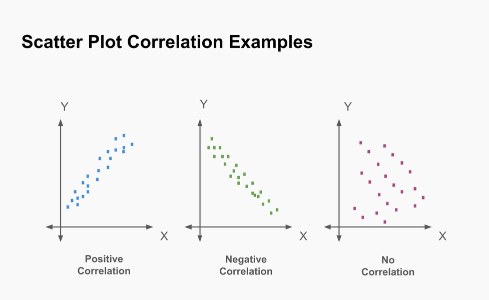
Example of a scatter plot showing data distribution.

A scatter plot visually represents the relationship between two variables, aiding in the selection of the appropriate correlation method.

Deep Dive: The Importance of Relationship Type

Understanding the distinction between linear and monotonic relationships is paramount when choosing between Pearson's and Spearman's correlation. A linear relationship implies a constant rate of change between variables, meaning if one variable increases by a certain amount, the other variable changes by a consistent, predictable amount. This is often seen in physical laws or well-controlled experiments. For instance, the relationship between the distance traveled and time at a constant speed is perfectly linear.

Conversely, a monotonic relationship simply means that as one variable increases, the other variable either consistently increases or consistently decreases, but not necessarily at a constant rate. The curve might be steep at some points and flat at others. For example, the relationship between advertising spend and sales might be monotonic but non-linear, where initial advertising brings significant sales increases, but subsequent spending yields diminishing returns.

This video provides a clear comparison of Pearson vs Spearman Correlation, focusing on assumptions and graph interpretations. It is highly relevant for understanding the visual differences in the types of relationships each coefficient measures, offering a practical perspective on their application.

Assessing Correlation Method Suitability: A Radar Chart Analysis

To further illustrate the practical considerations when choosing between Pearson's and Spearman's correlation, consider the suitability of each method across various analytical dimensions. This radar chart provides an opinionated analysis of their strengths and weaknesses in common research scenarios.

As depicted in the radar chart, Pearson's correlation excels in scenarios requiring high precision for continuous, linearly related data, but its sensitivity to outliers and strict distributional assumptions are notable limitations. Conversely, Spearman's correlation demonstrates superior robustness to outliers and flexibility with data distributions, making it highly suitable for ordinal data or when linearity is not guaranteed. However, it sacrifices some precision for strictly linear, continuous relationships by operating on ranks.

Navigating the Decision: A Mindmap for Choosing Correlation

The process of selecting the appropriate correlation coefficient can be simplified by following a decision-making framework. This mindmap outlines the key considerations and paths leading to either Pearson's or Spearman's correlation.

mindmap root["Choosing Correlation Method"] id1["Type of Relationship?"] id2["Linear?"] id3["Yes"] id4["Data Type & Distribution?"] id5["Continuous & Normal?"] id6["Yes"] id7["Outliers Present?"] id8["No"] id9["Pearson's Correlation"] id10["Yes"] id11["Consider Spearman's or data transformation"] id12["No"] id13["Spearman's Correlation"] id14["Monotonic (but not necessarily linear)?"] id15["Yes"] id16["Spearman's Correlation"] id17["No (e.g., U-shaped, complex)"] id18["Other statistical methods (e.g., Regression, ANOVA)"] id19["Data Scale?"] id20["Interval/Ratio (Continuous)?"] id21["Pearson's (if assumptions met)
or Spearman's (if assumptions violated)"] id22["Ordinal (Ranked)?"] id23["Spearman's Correlation"] id24["Sensitivity to Outliers?"] id25["Sensitive (need robustness)"] id26["Spearman's Correlation"] id27["Not sensitive (data clean)"] id28["Pearson's (if assumptions met)"]

This mindmap illustrates that the initial step in choosing a correlation method involves identifying the expected type of relationship between your variables. If a linear relationship is anticipated, further checks on data type, distribution, and outlier presence will guide you towards Pearson's or a cautious use of Spearman's. If the relationship is monotonic but not strictly linear, or if your data is ordinal or non-normally distributed, Spearman's emerges as the more appropriate choice.

Frequently Asked Questions

What are the main output values of Pearson's and Spearman's correlation?

Both Pearson's 'r' and Spearman's 'ρ' (rho) produce a correlation coefficient ranging from -1 to +1. A value of +1 indicates a perfect positive correlation, -1 indicates a perfect negative correlation, and 0 indicates no relationship. The difference lies in the type of relationship they quantify (linear vs. monotonic).

Can I use Pearson's correlation if my data is not normally distributed?

While Pearson's correlation technically assumes normal distribution, it can be somewhat robust to minor deviations, especially with large sample sizes. However, for significantly non-normal data or if outliers are present, Spearman's correlation is generally a more robust and appropriate choice. Visualizing your data with a histogram or Q-Q plot can help assess normality.

When should I choose Spearman's over Pearson's?

Choose Spearman's correlation when: 1) your data is ordinal (ranked), 2) your continuous data is not normally distributed, 3) there are significant outliers in your data, or 4) you expect a monotonic but not necessarily linear relationship between your variables. It is a non-parametric alternative that provides a robust measure of association in these scenarios.

Do I need to calculate ranks manually for Spearman's correlation?

No, most statistical software packages (like R, Python with libraries like SciPy, SPSS, or Jamovi) can automatically convert your raw data into ranks and compute Spearman's correlation for you. Understanding the ranking process is crucial for interpretation, but manual calculation is rarely necessary in practice.

Conclusion

In summary, both Pearson's Product Moment Correlation and Spearman's Rank-Order Correlation are indispensable tools for understanding relationships between variables, yet they serve different analytical purposes. Pearson's is the preferred method for quantifying strong, linear associations between continuous, normally distributed variables, providing precise insights into proportional changes. In contrast, Spearman's offers a more flexible and robust approach, suitable for monotonic relationships, ordinal data, or continuous data that do not meet the strict assumptions of normality and linearity, particularly in the presence of outliers. The judicious selection of either coefficient depends on the inherent characteristics of your data and the specific nature of the relationship you aim to investigate.