Unraveling Statistical Relationships: Pearson vs. Spearman Correlation

Key Insights into Correlation Analysis

Pearson's Product Moment Correlation measures the strength and direction of a linear relationship between two continuous variables, assuming normality and sensitivity to outliers.
Spearman's Rank-Order Correlation assesses the strength and direction of a monotonic relationship (consistent but not necessarily linear) between two variables, suitable for ordinal data or non-normal continuous data, and is robust to outliers.
The choice between Pearson's and Spearman's hinges on the type of relationship expected, the nature of the data (continuous vs. ordinal), and the presence of outliers or non-normality.

In the realm of statistical analysis, understanding the relationship between two variables is paramount. Two of the most widely used statistical measures for this purpose are Pearson’s Product Moment Correlation Coefficient (often denoted as Pearson’s r or PMCC) and Spearman’s Rank-Order Correlation Coefficient (typically denoted as Spearman’s ρ or r_s). While both coefficients quantify the strength and direction of an association between two variables, they operate under distinct assumptions, are best suited for different types of data, and capture different forms of relationships. This comprehensive discussion will delve into their fundamental differences, computational approaches, strengths, weaknesses, and practical applications, supported by illustrative examples.

Defining the Core: Linear vs. Monotonic Relationships

The primary distinction between Pearson's and Spearman's correlation lies in the type of relationship they are designed to detect. Visualizing the relationship between variables using scatter plots is often recommended before selecting a coefficient, as it can clearly indicate whether a linear or monotonic trend is more appropriate.

Pearson's Product Moment Correlation: The Linear Litmus Test

Pearson's r is a parametric statistical measure that quantifies the strength and direction of a linear relationship between two continuous variables. A linear relationship implies that as one variable increases or decreases, the other variable changes by a consistent, constant amount, forming a straight line on a scatter plot. The coefficient ranges from -1 to +1:

+1: Indicates a perfect positive linear relationship (as one variable increases, the other increases proportionally).
-1: Indicates a perfect negative linear relationship (as one variable increases, the other decreases proportionally).
0: Suggests no linear relationship between the variables.

Pearson's correlation is calculated based on the raw numerical values of the data, taking into account their means and standard deviations. It is particularly useful when variables are expected to exhibit a direct, proportional relationship.

Spearman's Rank-Order Correlation: Capturing Consistent Trends

Spearman's ρ, conversely, is a non-parametric measure that assesses the strength and direction of a monotonic relationship between two variables. A monotonic relationship means that as one variable increases, the other consistently either increases or decreases, but not necessarily at a constant rate or in a straight line. In essence, it is the Pearson correlation calculated on the ranks of the data rather than their actual values. This makes Spearman's robust to non-linear but consistent trends.

+1: Signifies a perfect positive monotonic relationship (as one variable's rank increases, the other's rank consistently increases).
-1: Signifies a perfect negative monotonic relationship (as one variable's rank increases, the other's rank consistently decreases).
0: Indicates no monotonic relationship between the ranks of the variables.

Because it operates on ranks, Spearman's is highly versatile and can detect associations even when the relationship is curved or non-linear, as long as the direction of change is consistent.

Navigating Data Types and Assumptions

The choice between Pearson's and Spearman's is heavily influenced by the nature of the data and the underlying statistical assumptions that each coefficient demands.

Pearson's Assumptions: A Strict Linear Framework

Pearson's r comes with several strict assumptions that, if violated, can lead to inaccurate or misleading conclusions:

Continuous Variables:
Both variables must be continuous (interval or ratio scale), meaning they can take on any value within a given range (e.g., temperature, height, income).
Linearity:
The relationship between the two variables must be linear. If the relationship is genuinely curvilinear, Pearson's r might underestimate the actual association.
Normal Distribution:
The variables should be approximately normally distributed (bivariate normality). While minor deviations may be tolerable, significant skewness can affect the accuracy.
Homoscedasticity:
The variance of one variable should be roughly constant across all levels of the other variable.
Absence of Outliers:
Pearson's r is highly sensitive to outliers, which are extreme values that can disproportionately influence the mean and standard deviation, thereby skewing the correlation coefficient. A single outlier can significantly alter the perceived strength and even direction of a linear relationship.

Spearman's Flexibility: Embracing Ranks

Spearman's ρ is far less restrictive regarding assumptions, making it a powerful alternative when Pearson's criteria are not met:

Ordinal, Interval, or Ratio Data:
It is ideal for ordinal data (ranked data like survey responses on a Likert scale: "strongly disagree," "disagree," etc.). It can also be applied to continuous data (interval or ratio) by converting them into ranks, which is particularly useful when these continuous data do not meet Pearson's normality assumptions or contain outliers.
Monotonicity:
The primary assumption is that the relationship between the variables is monotonic.
Non-parametric Nature:
As a non-parametric test, Spearman's does not require the data to be normally distributed. This makes it more robust for skewed distributions or smaller sample sizes.
Robustness to Outliers:
Because it transforms raw data into ranks, extreme values have a reduced impact. The rank of an outlier will still be an extreme rank, but its exact magnitude (which is what Pearson's uses) is neutralized, making Spearman's less sensitive to them.

Consider the visualization below. Scatter plots are invaluable for discerning the type of relationship present. A perfectly straight line suggests Pearson's, while a consistently increasing or decreasing curve points towards Spearman's.

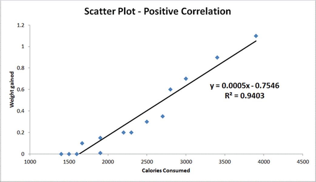
An example of a scatter plot showing a positive linear correlation, which is suitable for Pearson's analysis.

Mathematical Foundations and Interpretations

Understanding the underlying formulas clarifies why each coefficient behaves differently and what its value signifies.

Pearson's Formula: Covariance in Action

Pearson's r is computed using the covariance of the two variables, divided by the product of their standard deviations. This formula directly incorporates the raw values of the data:

\[ r = \frac{\sum (X_i - \bar{X})(Y_i - \bar{Y})}{\sqrt{\sum (X_i - \bar{X})^2 \sum (Y_i - \bar{Y})^2}} \]

Where \(X_i\) and \(Y_i\) are individual data points, and \(\bar{X}\) and \(\bar{Y}\) are their respective means. This "product moment" approach is sensitive to the magnitude of values and their distances from the mean, explaining its sensitivity to outliers.

Spearman's Formula: Rank Differences

Spearman's ρ is essentially the Pearson correlation coefficient applied to the ranks of the observations instead of their raw values. A simplified formula is often used when there are no tied ranks:

\[ r_s = 1 - \frac{6 \sum d_i^2}{n(n^2 - 1)} \]

Where \(d_i\) is the difference between the ranks of each pair of observations, and \(n\) is the number of pairs. When there are tied ranks, more complex methods are used, but the principle remains the same: it assesses the correlation between the ranks.

Interpreting the Coefficients: A Range of -1 to +1

Both Pearson's r and Spearman's ρ yield values between -1 and +1:

A value close to +1 indicates a strong positive correlation (either linear for Pearson's, or monotonic for Spearman's).
A value close to -1 indicates a strong negative correlation.
A value close to 0 suggests a weak or no relationship of the type measured by the coefficient.

Crucially, a Pearson's r of ±1 implies a perfect linear relationship, meaning all data points fall exactly on a straight line. Conversely, a Spearman's ρ of ±1 indicates a perfect monotonic relationship, where the ranks are perfectly ordered, but the actual values do not necessarily form a straight line.

When to Use Which: Practical Decision-Making

The decision to use Pearson's or Spearman's correlation depends heavily on the characteristics of your data and the research question. Here's a quick guide:

Characteristic	Pearson’s Product Moment Correlation (r)	Spearman’s Rank-Order Correlation (ρ or r_s)
Relationship Measured	Linear relationships	Monotonic relationships (linear or non-linear, but consistently directional)
Data Type	Continuous (interval or ratio scale)	Ordinal, or continuous data with violated assumptions
Assumptions	Linearity, normal distribution, homoscedasticity, absence of outliers	Monotonicity, data can be ranked; no strict distribution assumptions
Sensitivity to Outliers	Highly sensitive	Less sensitive (due to rank transformation)
Parametric / Non-parametric	Parametric test	Non-parametric test
Typical Application	Evaluating direct linear associations between quantitative variables (e.g., height vs. weight)	Assessing trends in ranked data, or when data is not normally distributed (e.g., survey responses, expert rankings)

Illustrative Examples and Applications

Let's solidify the understanding with specific examples:

Example 1: Temperature and Chocolate Coating Thickness (Pearson's Domain)

A chocolate factory wants to determine if there's a linear relationship between the ambient temperature in the production facility and the thickness of the chocolate coating on their products. If both temperature and thickness are continuous variables that are approximately normally distributed, and preliminary scatter plots suggest a straight-line relationship (e.g., as temperature increases, coating thickness consistently decreases), Pearson's r would be the appropriate choice. A high negative Pearson's r (e.g., -0.85) would indicate a strong inverse linear relationship, meaning higher temperatures are linearly associated with thinner coatings.

Example 2: Employee Test Order and Tenure (Spearman's Domain)

A company wants to assess whether the order in which employees complete a new test is related to their tenure (number of months employed). The "order of completion" is ordinal data, and "months employed" is continuous but might not be normally distributed, or the relationship might not be strictly linear. Spearman's ρ is ideal here. If employees with longer tenure tend to complete the test earlier, even if not at a perfectly linear rate, a high negative Spearman's ρ (e.g., -0.7) would indicate a strong monotonic relationship between higher tenure and earlier completion ranks.

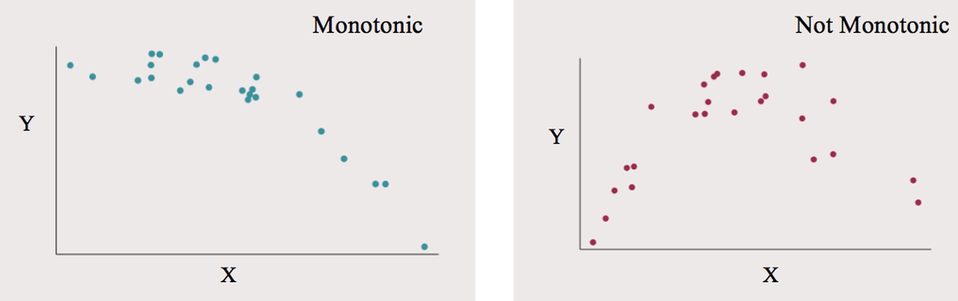
Illustrations of monotonic relationships, which Spearman's correlation can effectively measure, even when not perfectly linear.

Example 3: Income and Happiness (Comparative Scenario)

Consider a study exploring the relationship between an individual's income and their self-reported happiness level (on a scale of 1-10). While income is continuous, happiness ratings are ordinal, and the relationship might be monotonic but non-linear (e.g., happiness increases sharply with initial income gains but then plateaus). In this case, Spearman's ρ would likely provide a more accurate measure of the association. Pearson's r might yield a lower coefficient, underestimating the true correlation due to the non-linear nature, whereas Spearman's ρ would capture the consistent trend of higher income generally correlating with higher happiness ranks, even if the exact increments aren't linear.

Visualizing Correlation Metrics

To further illustrate the comparative strengths and weaknesses of Pearson's and Spearman's correlation, we can use a radar chart. This chart will visually represent how each coefficient performs across various data characteristics and relationship types, based on our analytical insights.

As illustrated by the radar chart, Pearson's excels in accurately measuring linear relationships and when data adheres strictly to normality. However, its performance drops when dealing with outliers, ordinal data, or when assumptions are relaxed. Conversely, Spearman's shines in its ability to capture monotonic trends, its robustness to outliers, and its flexibility with various data types, especially ordinal and non-normal distributions, though it sacrifices some precision when the relationship is perfectly linear and parametric assumptions hold.

A Mindmap of Correlation Concepts

To provide a structured overview of the decision-making process when choosing between Pearson's and Spearman's correlation, here is a mindmap. It highlights the key considerations and paths based on data characteristics and relationship types.

mindmap root["Correlation Coefficient Choice"] Pearson["Pearson's Product Moment Correlation"] Pearson-->P1["Measures LINEAR relationships"] Pearson-->P2["Requires:"] P2-->P2a["Continuous variables"] P2a-->P2a1["Interval or Ratio scale"] P2-->P2b["Approximately Normal Distribution"] P2-->P2c["No significant Outliers"] P2-->P2d["Homoscedasticity"] Pearson-->P3["Sensitive to Outliers"] Pearson-->P4["Parametric Test"] Spearman["Spearman's Rank-Order Correlation"] Spearman-->S1["Measures MONOTONIC relationships"] S1-->S1a["Can be linear or non-linear"] Spearman-->S2["Suitable for:"] S2-->S2a["Ordinal Data"] S2-->S2b["Continuous Data (non-normal)"] S2-->S2c["Presence of Outliers"] Spearman-->S3["Less sensitive to Outliers"] Spearman-->S4["Non-parametric Test"] Spearman-->S5["Calculated on Ranks"] Decision["Decision Criteria"] Decision-->D1["Type of Relationship?"] D1-->D1a["Linear --> Pearson"] D1-->D1b["Monotonic --> Spearman"] Decision-->D2["Data Distribution?"] D2-->D2a["Normal --> Pearson (if other assumptions met)"] D2-->D2b["Non-normal --> Spearman"] Decision-->D3["Outliers Present?"] D3-->D3a["Yes --> Spearman"] D3-->D3b["No --> Both possible"] Decision-->D4["Data Type?"] D4-->D4a["Continuous (Interval/Ratio) --> Both (check assumptions)"] D4-->D4b["Ordinal --> Spearman"]

This mindmap serves as a quick reference, guiding you through the key considerations when selecting the appropriate correlation coefficient based on your data and research objectives. It highlights that understanding the nature of your variables and the expected relationship is paramount.

Deep Dive: Practical Demonstration of Correlation

To further illustrate the concepts discussed, this video offers a clear explanation of both Pearson and Spearman correlations, including their graph interpretations. Watching this visual guide can greatly enhance your understanding of how these statistical measures are applied and what their results visually represent.

An insightful video explaining Pearson Correlation vs Spearman Correlation with clear graph interpretations.

This video is particularly relevant because it visually demonstrates the difference between linear and monotonic relationships through scatter plots, making it easier to grasp why one coefficient might be more suitable than the other in different scenarios. It bridges the gap between theoretical understanding and practical application, showing how varying data distributions affect the correlation outcome for both Pearson's and Spearman's.

Frequently Asked Questions (FAQ)

What is the main difference between Pearson’s and Spearman’s correlation?

The main difference lies in the type of relationship they measure: Pearson’s measures linear relationships between continuous variables, while Spearman’s measures monotonic (consistently increasing or decreasing, but not necessarily linear) relationships, suitable for ordinal data or non-normal continuous data.

When should I use Pearson’s correlation?

Use Pearson’s correlation when you have two continuous variables, expect a linear relationship, and your data is approximately normally distributed with no significant outliers. It provides a precise measure of the strength and direction of this linear association.

When should I use Spearman’s correlation?

Use Spearman’s correlation when your data is ordinal, or when your continuous data is not normally distributed, contains outliers, or when you expect a monotonic but potentially non-linear relationship. It's a non-parametric alternative that works by ranking the data.

Are correlation coefficients sensitive to outliers?

Yes, Pearson’s correlation is highly sensitive to outliers because it uses the raw data values in its calculation. Spearman’s correlation, by contrast, is less sensitive to outliers because it transforms the data into ranks, reducing the impact of extreme values.

Can Spearman’s correlation be used for continuous data?

Yes, Spearman’s correlation can be used for continuous data. In such cases, the continuous data is first converted into ranks, and then the correlation is calculated based on these ranks. This approach is particularly useful if the continuous data does not meet the normality assumptions required for Pearson’s, or if there are significant outliers.

Conclusion

In summary, both Pearson’s Product Moment Correlation and Spearman’s Rank-Order Correlation are indispensable tools in statistical analysis, each serving a distinct purpose. Pearson’s r is the go-to for assessing the strength and direction of strict linear relationships between continuous, normally distributed variables. Its precision in capturing linearity makes it powerful when its assumptions are met. Spearman’s ρ, on the other hand, offers greater versatility and robustness, excelling in scenarios involving ordinal data, non-normal distributions, or when the relationship is monotonic but not strictly linear. By converting data to ranks, it effectively mitigates the influence of outliers. The judicious selection of either coefficient is crucial for drawing accurate and meaningful conclusions from data, necessitating a careful consideration of the data type, distribution, presence of outliers, and the suspected nature of the relationship between variables. Understanding these distinctions ensures that researchers and analysts apply the most appropriate statistical measure for their specific analytical needs.