---

Key Highlights

• Calculating Probability: Determining the likelihood of a bulb having a lifespan less than 2000 hours using the normal distribution.
• Applications of Probability Theory: Understanding the broad use of probability in risk assessment, forecasting, and decision-making across various fields.
• Objective vs. Subjective Probability: Differentiating between probabilities based on empirical data and personal beliefs.

---

Calculating the Probability of Bulb Lifespan

To determine the probability that a randomly selected bulb will have a lifespan of less than 2000 hours, we need to use the concepts of normal distribution and z-scores. Here’s how we can approach this:

Understanding the Normal Distribution

The normal distribution, often called the bell curve, is a common probability distribution. It's symmetrical around the mean, indicating that data near the mean are more frequent than data far from the mean. The standard deviation measures the dispersion or spread of the data around the mean.

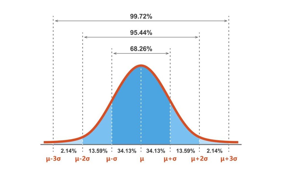
In this case, the mean lifespan \( \mu \) is 3000 hours, and the standard deviation \( \sigma \) is 400 hours.

Calculating the Z-Score

The z-score tells us how many standard deviations an element is from the mean. It is calculated using the formula:

\[ z = \frac{x - \mu}{\sigma} \]

Where:

• \( x \) is the value we are interested in (2000 hours)
• \( \mu \) is the mean (3000 hours)
• \( \sigma \) is the standard deviation (400 hours)

Plugging in the values:

\[ z = \frac{2000 - 3000}{400} = -2.5 \]

This means that 2000 hours is 2.5 standard deviations below the mean.

Finding the Probability

We need to find the probability \( P(X < 2000) \), which is equivalent to finding the area under the normal distribution curve to the left of \( z = -2.5 \). Using a standard normal distribution table or a calculator, we find that the probability corresponding to a z-score of -2.5 is approximately 0.0062.

Therefore, the probability that a randomly selected bulb will have a lifespan of less than 2000 hours is approximately 0.62%.

---

Situations Where Probability Theory is Essential

Probability theory is a fundamental tool in numerous fields, helping to quantify and manage uncertainty. Here are some key areas where it plays a crucial role:

Risk Assessment and Management

In finance and insurance, probability theory is used to assess the likelihood of various events, such as market crashes, natural disasters, or health issues. Actuarial science relies heavily on probability to calculate insurance premiums and manage risk.

Forecasting and Prediction

Probability is used in weather forecasting, economic predictions, and sales forecasting. By analyzing historical data and applying probability models, analysts can estimate future outcomes.

Decision Making

In business and engineering, probability theory helps in making informed decisions. For example, in quality control, it is used to determine the probability of defects in a production line. In investment, it aids in evaluating the potential returns and risks of different investment options.

Medical Field

Probability theory helps understand and control the spread of diseases using genetics and heuristics. It is used for medical purposes to understand the spread of diseases.

---

Understanding Sample Space, Sample Points, and Events

In probability theory, it's crucial to understand the concepts of sample space, sample points, and events. These form the foundation for calculating probabilities and understanding random phenomena.

Sample Space

The sample space, often denoted as \( S \), is the set of all possible outcomes of a random experiment. For example, if we toss a coin, the sample space is \( S = \{ \text{Heads, Tails} \} \). If we roll a six-sided die, the sample space is \( S = \{1, 2, 3, 4, 5, 6 \} \).

Sample Points

Each element in the sample space is called a sample point. In the coin toss example, "Heads" and "Tails" are sample points. In the die rolling example, each number from 1 to 6 is a sample point.

Events

An event is a subset of the sample space. It is a collection of one or more sample points. For example, if we roll a die, an event could be "rolling an even number," which corresponds to the subset \( \{2, 4, 6 \} \) of the sample space \( \{1, 2, 3, 4, 5, 6 \} \). Another event could be "rolling a number greater than 4," which corresponds to the subset \( \{5, 6 \} \).

Example: Bulb Lifespan

In the context of the bulb lifespan problem:

• Sample Space: The set of all possible lifespans of the bulbs, which could be any non-negative real number (though practically, it would be within a reasonable range, say 0 to 5000 hours).
• Sample Points: Each individual lifespan value, such as 2000 hours, 3000 hours, etc.
• Event: The event of interest is the bulb having a lifespan less than 2000 hours.

---

Objective vs. Subjective Probability

Probability can be interpreted in different ways, leading to the distinction between objective and subjective probability.

Objective Probability

Objective probability is based on empirical evidence and can be verified through observation or experimentation. There are two main types of objective probability:

• Classical Probability: This is based on the assumption that all outcomes in the sample space are equally likely. For example, the probability of getting heads when tossing a fair coin is \( \frac{1}{2} \), because there are two equally likely outcomes.
• Empirical Probability: This is based on observed data from repeated trials. For example, if a factory produces 1000 light bulbs and 10 are defective, the empirical probability of a bulb being defective is \( \frac{10}{1000} = 0.01 \).

Subjective Probability

Subjective probability, also known as Bayesian probability, is based on personal beliefs, experiences, or judgments. It reflects an individual's degree of confidence in an event occurring. Unlike objective probability, subjective probability cannot be verified through experimentation and may vary from person to person. For example, an expert might assess the probability of a new technology succeeding based on their knowledge and experience.

Key Differences

The main differences between objective and subjective probability are summarized in the table below:

Feature	Objective Probability	Subjective Probability
Basis	Empirical evidence, observed data	Personal beliefs, judgments
Verification	Can be verified through experimentation	Cannot be directly verified
Variability	Generally consistent across individuals	May vary from person to person
Use Cases	Scientific research, statistical analysis, insurance	Business decisions, strategic planning, risk assessment

---

FAQ

What is probability theory?

Probability theory is the branch of mathematics that deals with quantifying uncertainty. It provides a framework for analyzing random events and predicting their likelihood of occurrence.

How is probability used in weather forecasting?

Meteorologists use probability theory to assess the likelihood of different weather conditions, such as rain, snow, or sunshine. They analyze historical weather data and current atmospheric conditions to create probabilistic forecasts.

What is a normal distribution?

A normal distribution, also known as a bell curve, is a common probability distribution that is symmetrical around the mean. It is characterized by its mean and standard deviation, which determine the center and spread of the distribution, respectively.

How do insurance companies use probability?

Insurance companies use probability theory to estimate the likelihood of various events, such as car accidents, fires, or illnesses. This helps them determine appropriate insurance premiums and manage their risk exposure.

Can subjective probability be useful?

Yes, subjective probability can be useful in situations where objective data is limited or unavailable. It allows decision-makers to incorporate their personal beliefs and experiences into the decision-making process, especially in areas like strategic planning and risk assessment.

---

References

Last updated April 11, 2025