Unveiling the Lifespan Odds: How Likely Is an Early Bulb Burnout?

Calculating the chances of a short lifespan and exploring the foundations of probability theory.

Understanding the probability of events, like a light bulb failing earlier than expected, is crucial in many fields. This involves applying statistical concepts to predict outcomes based on known data. Let's break down the probability calculation for the bulb's lifespan and delve into the core ideas of probability theory.

Highlights

Specific Bulb Probability: The probability of a randomly selected bulb lasting less than 2000 hours, given a mean life of 3000 hours and a standard deviation of 400 hours, is approximately 0.62%.
Probability Theory's Reach: This mathematical framework is essential for analyzing uncertainty, managing risk, and making informed decisions in diverse areas like finance, engineering, medicine, and data science.
Objective vs. Subjective Probability: Objective probability relies on measurable data and frequencies, while subjective probability is based on personal beliefs and judgments.

Calculating the Probability of a Short Lifespan

We are given that the lifespan of the bulbs follows a normal distribution with:

Mean (μ) = 3000 hours
Standard Deviation (σ) = 400 hours

We want to find the probability that a randomly selected bulb has a lifespan (X) less than 2000 hours, denoted as P(X < 2000).

Step 1: Standardization using the Z-score

To determine this probability using the standard normal distribution, we first convert the value of 2000 hours into a Z-score. The Z-score tells us how many standard deviations a particular value is away from the mean.

The formula for the Z-score is:

\[ Z = \frac{X - \mu}{\sigma} \]

Plugging in the values:

\[ Z = \frac{2000 \, \text{hours} - 3000 \, \text{hours}}{400 \, \text{hours}} = \frac{-1000}{400} = -2.5 \]

A Z-score of -2.5 means that a lifespan of 2000 hours is 2.5 standard deviations below the mean lifespan of 3000 hours.

Step 2: Finding the Probability from the Z-score

Now, we need to find the probability corresponding to a Z-score less than -2.5. This represents the area under the standard normal distribution curve to the left of Z = -2.5.

Using a standard normal distribution table or a statistical calculator, we find:

\[ P(Z < -2.5) \approx 0.0062 \]

Therefore, the probability that a randomly selected bulb will have a mean life of less than 2000 hours is approximately 0.0062, or 0.62%.

When Do We Need Probability Theory?

Probability theory is the mathematical language of uncertainty. It's indispensable whenever we need to quantify the likelihood of different outcomes, analyze randomness, or make decisions in the face of incomplete information. Its applications span numerous domains:

Risk Management and Finance

Assessing and mitigating risks is central to insurance and finance. Probability helps in:

Calculating insurance premiums based on the likelihood of claims (e.g., accidents, health issues).
Modeling financial market fluctuations and predicting stock price movements.
Evaluating the risk associated with investments.

Science and Engineering

From designing experiments to ensuring product quality, probability is fundamental:

Assessing the reliability and lifespan of components (like the light bulb example).
Quality control in manufacturing processes to minimize defects.
Modeling complex physical systems (e.g., particle physics, thermodynamics).
Analyzing experimental data and testing scientific hypotheses.
Predicting weather patterns and natural disaster occurrences.

Medicine and Biology

Understanding biological processes and medical outcomes often involves probability:

Evaluating the effectiveness of new treatments in clinical trials.
Assessing the probability of disease occurrence based on risk factors or genetic markers.
Modeling the spread of infectious diseases (epidemiology).

Data Science, AI, and Computing

Probability forms the backbone of many modern computational techniques:

Developing algorithms for machine learning (e.g., Naive Bayes classifiers, Bayesian networks).
Building spam filters and recommendation systems.
Analyzing network traffic and system performance.
Underpinning statistical inference and data analysis methods.

Everyday Decisions and Games

Even outside formal settings, probabilistic thinking helps:

Understanding odds in games of chance (like lotteries or card games).
Making informed choices based on uncertain forecasts (e.g., planning an outdoor event based on rain probability).
Evaluating sports outcomes and betting odds.

Core Concepts: Sample Space, Sample Points, and Events

To work with probability formally, we use a few key concepts to structure our thinking about random phenomena or experiments.

Sample Space (Ω)

The sample space is the foundational set containing all possible outcomes of a random experiment. It represents the universe of possibilities for that specific experiment.

Example (Coin Toss): The sample space is {Heads, Tails}.
Example (Rolling a Die): The sample space is {1, 2, 3, 4, 5, 6}.
Example (Bulb Lifespan): The sample space consists of all possible non-negative lifespan durations, theoretically [0, ∞) hours. This is a continuous sample space.

Sample Points

Sample points are the individual outcomes within the sample space. Each element listed in the sample space is a sample point.

Example (Coin Toss): 'Heads' is a sample point, and 'Tails' is another sample point.
Example (Rolling a Die): The number '4' is a sample point.
Example (Bulb Lifespan): A specific lifespan, like 3150.7 hours, is a sample point. In continuous spaces, there are infinitely many sample points.

Events (E)

An event is a subset of the sample space. It represents a specific result or a collection of results we might be interested in. An event occurs if the outcome of the experiment is one of the sample points in that subset.

Example (Coin Toss): The event "getting Heads" corresponds to the subset {Heads}.
Example (Rolling a Die): The event "rolling an even number" corresponds to the subset {2, 4, 6}. The event "rolling a number greater than 4" corresponds to {5, 6}.
Example (Bulb Lifespan): The event "the bulb lasts less than 2000 hours" corresponds to the subset of all sample points (lifespans) between 0 and 2000 hours, i.e., the interval [0, 2000).

Probability theory assigns a numerical value (between 0 and 1) to events, indicating how likely they are to occur.

Visualizing Probability Concepts

This mindmap illustrates the relationship between the core concepts of probability theory, from the initial experiment to applications and types of probability.

mindmap root["Probability Theory"] ["Core Concepts"] ["Random Experiment"] ["(e.g., Measuring Bulb Life)"] ["Sample Space (Ω)"] ["(Set of all outcomes)"] ["e.g., {Heads, Tails}"] ["e.g., {Lifespan ≥ 0 hours}"] ["Sample Points"] ["(Individual outcomes)"] ["e.g., Heads"] ["e.g., 2950 hours"] ["Events (E)"] ["(Subset of Ω)"] ["e.g., {Heads}"] ["e.g., {Lifespan < 2000 hours}"] ["Types of Probability"] ["Objective"] ["Based on Data/Frequency"] ["Factual & Reproducible"] ["Subjective"] ["Based on Belief/Judgment"] ["Personal & Variable"] ["Calculation & Analysis"] ["Probability Value P(E)"] ["(0 ≤ P(E) ≤ 1)"] ["Distributions (e.g., Normal)"] ["Mean (μ)"] ["Standard Deviation (σ)"] ["Z-Score"] ["Applications"] ["Risk Management"] ["Science & Engineering"] ["Data Analysis & AI"] ["Decision Making"] ["Forecasting"]

Objective vs. Subjective Probability: Data vs. Belief

Probability quantifies likelihood, but the way we arrive at that quantification can differ. The main distinction lies between objective and subjective approaches.

Objective Probability

Objective probability is determined based on empirical evidence, historical data, logical analysis, or symmetrical outcomes. It relies on repeatable processes and observable frequencies.

Basis: Frequencies from long-run experiments, mathematical models, physical symmetries (like a fair die).
Nature: Factual, verifiable, and generally agreed upon given the same evidence. It aims to be free from personal bias.
Example: The probability of getting heads when flipping a fair coin is 0.5. The calculated probability of the bulb lasting less than 2000 hours (0.0062) is objective, assuming the mean and standard deviation are accurate population parameters or derived from large samples.

Subjective Probability

Subjective probability represents an individual's degree of belief or confidence in the occurrence of an event. It's based on personal judgment, experience, intuition, and available (possibly incomplete) information.

Basis: Personal assessment, expert opinion, educated guesses, feelings.
Nature: Personal, varies from person to person, can be influenced by biases. It's often used when empirical data is scarce or unique situations arise.
Example: A sports analyst estimating the probability of a specific team winning the championship based on their knowledge of players, recent performance, and gut feeling. An investor assessing the likelihood of a startup's success based on their impression of the founders.

Comparing the Two Approaches

The table below summarizes the key differences:

Feature	Objective Probability	Subjective Probability
Basis	Empirical data, frequencies, logical models	Personal belief, intuition, judgment
Nature	Factual, verifiable, reproducible	Opinion-based, variable, personal
Source	Observed evidence, mathematical calculation	Experience, educated guesses, feelings
Consistency	Consistent across observers given the same data/model	Varies between individuals
Example	Probability of rolling a 6 on a fair die (1/6)	Estimating the chance of rain based on how the sky looks
Primary Use	Scientific research, engineering, quality control, games of chance	Personal decisions, unique events, preliminary estimates, Bayesian inference

Comparing Probability Types: A Visual Perspective

This radar chart visually compares objective and subjective probability across several key dimensions. Objective probability scores high on factors related to data and reproducibility, while subjective probability is characterized by personal influence.

Understanding Objective vs. Subjective Probability

This video provides a clear explanation of the core differences between objective probability, which is based on frequencies and data, and subjective probability, which stems from personal beliefs.

The distinction is crucial. Objective probabilities are preferred in scientific and engineering contexts like analyzing bulb lifespans because they offer consistency and are grounded in measurable evidence. Subjective probabilities, while useful for personal decision-making or situations with limited data, introduce variability based on individual perspectives.

Visualizing the Concepts: Light Bulbs and Distributions

The calculation we performed relies on the assumption that the light bulb lifespans follow a normal distribution, often depicted as a bell curve. The mean (3000 hours) represents the peak of the curve, and the standard deviation (400 hours) describes the spread. Our calculation found the area under this curve to the left of 2000 hours.

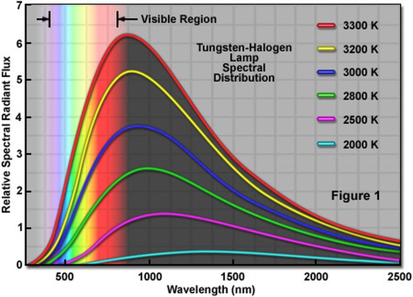
An example of a Tungsten-Halogen lamp, similar to the type of bulb whose lifespan might be analyzed using probability.

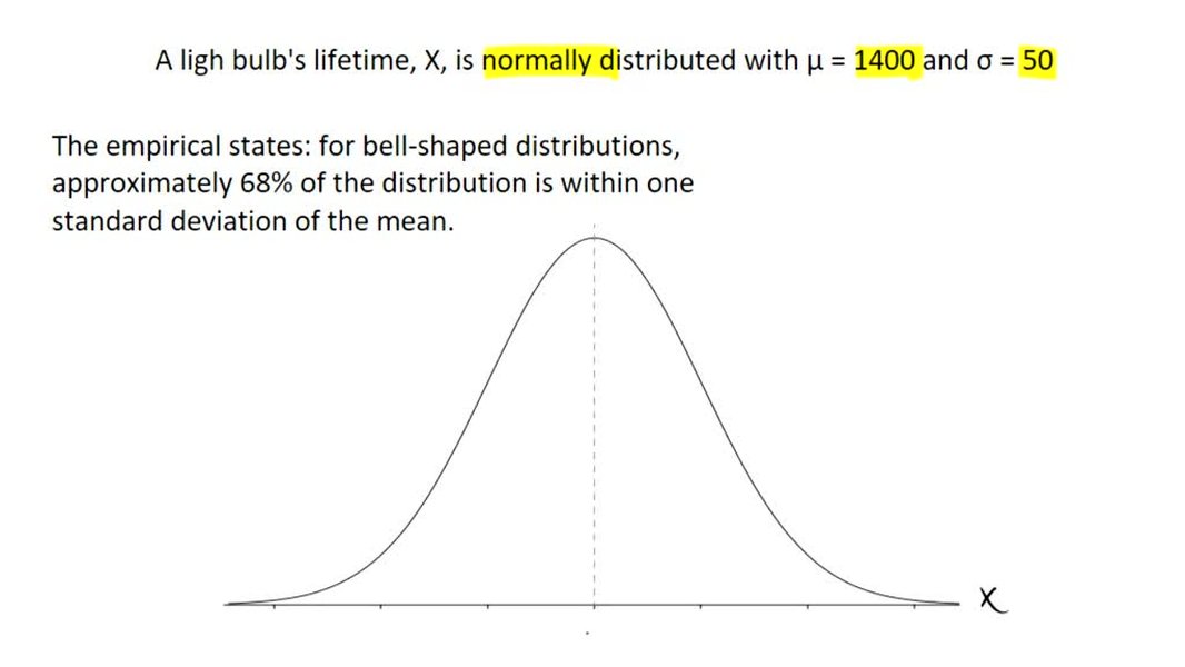
Normal Distribution Curve for Light Bulb Lifespan

Visual representation of a normal distribution curve, often used to model phenomena like light bulb lifespans. The shaded area would represent the probability of a bulb lasting less than a certain number of hours (e.g., 2000 hours in our case).

These images help connect the abstract concepts of probability and normal distributions to the tangible example of a light bulb's lifespan.

Frequently Asked Questions (FAQ)

What is a Z-score and why is it used?

A Z-score measures how many standard deviations a specific data point is away from the mean of its distribution. It standardizes values from different normal distributions, allowing them to be compared on a common scale (the standard normal distribution, which has a mean of 0 and a standard deviation of 1).

It's used because it allows us to easily calculate probabilities associated with any normally distributed variable using a single standard normal distribution table (Z-table) or calculator, regardless of the original mean and standard deviation.

\[ Z = \frac{\text{Data Point (X)} - \text{Mean (μ)}}{\text{Standard Deviation (σ)}} \]

Can probability be greater than 1 or less than 0?

No, probability values must always be between 0 and 1 (inclusive).

A probability of 0 means the event is impossible.
A probability of 1 means the event is certain to occur.
Probabilities between 0 and 1 represent varying degrees of likelihood.

If a calculation yields a probability outside this range, it indicates an error in the calculation or assumptions.

Is the normal distribution always applicable to real-world data like bulb life?

The normal distribution is a common and useful model, but it's not always a perfect fit for real-world data. Many natural phenomena and manufacturing processes tend to follow a normal distribution due to the Central Limit Theorem, especially when influenced by many small, random factors.

However, factors like manufacturing defects or specific failure modes can sometimes cause deviations from a perfect normal distribution. For bulb lifespans, while often approximated as normal, other distributions (like the Weibull distribution) might sometimes provide a better fit, especially when focusing on failure rates over time. Statistical tests are used to check if the normal distribution is an appropriate assumption for a given dataset.

How does probability theory relate to statistics?

Probability theory and statistics are closely related but distinct fields:

Probability Theory: Deals with predicting the likelihood of future events based on assumed models or parameters. It moves from general principles (the model) to specific outcomes (predictions). Example: *Given* a fair die, what is the probability of rolling a 6?
Statistics: Deals with analyzing observed data to infer properties of the underlying process or population. It moves from specific observations (data) to general principles (inferences about the model). Example: *Given* we rolled a die 100 times and got 30 sixes, is the die fair?

In essence, probability provides the mathematical foundation for statistical inference. Statistics uses probability to quantify the uncertainty in its conclusions drawn from data.