Calculating Probability of Light Bulb Lifespan and Understanding Probability Theory

Key Highlights

Probability Calculation: Determining the likelihood of a light bulb having a lifespan less than 2000 hours using normal distribution principles.
Applications of Probability Theory: Understanding how probability theory is essential in various fields like weather forecasting, insurance, and quantum mechanics.
Objective vs. Subjective Probability: Differentiating between probabilities based on empirical evidence and those based on personal beliefs.

Calculating the Probability of a Light Bulb's Lifespan

To calculate the probability that a randomly selected light bulb will have a lifespan of less than 2000 hours, given a mean life of 3000 hours and a standard deviation of 400 hours, we can use the standard normal distribution (Z-score). Here's how to approach it:

Calculate the Z-score:

The Z-score indicates how many standard deviations an element is from the mean. It is calculated using the formula: \[ Z = \frac{X - \mu}{\sigma} \] where \( X \) is the value of interest (2000 hours), \( \mu \) is the mean (3000 hours), and \( \sigma \) is the standard deviation (400 hours).

Plugging in the values: \[ Z = \frac{2000 - 3000}{400} = \frac{-1000}{400} = -2.5 \]

Find the Probability:

The Z-score of -2.5 corresponds to the area under the standard normal curve to the left of -2.5. Using a Z-table or a calculator, we find that the probability \( P(Z < -2.5) \) is approximately 0.0062.

Interpretation:

This means there is approximately a 0.62% chance that a randomly selected light bulb will have a lifespan of less than 2000 hours.

Applications of Probability Theory in Real-World Scenarios

Probability theory is fundamental in various fields, helping to quantify uncertainty and make informed decisions. Here are some key areas where it's applied:

Weather Forecasting

Meteorologists use probability to predict weather patterns. For example, the "chance of rain" is a probabilistic statement about the likelihood of precipitation in a given area.

Sports Analytics

Probability is used to predict the outcomes of sporting events, assess player performance, and develop game strategies. This includes calculating the likelihood of a team winning, a player scoring, or other specific events occurring during a game.

Insurance

Insurance companies rely heavily on probability theory to assess risk and determine premiums. They analyze historical data to estimate the likelihood of events such as car accidents, natural disasters, or health issues.

Finance and Investing

In finance, probability theory is used to model market behavior, assess investment risks, and make portfolio management decisions. It helps in estimating the potential returns and risks associated with different investment options.

Medical Decisions

Probability is crucial in medical research and clinical practice. It is used to assess the effectiveness of treatments, diagnose diseases, and predict patient outcomes.

Quantum Mechanics

Probability is intrinsic to quantum mechanics, where the behavior of particles is described in terms of probabilities. For instance, the probability of finding an electron in a particular location around an atom is a fundamental concept.

Games of Chance

Probability theory is the backbone of games of chance, such as card games, dice games, and lotteries. It helps in calculating the odds of winning and understanding the risks involved.

Sample Space, Sample Points, and Events in Probability Theory

Understanding the basic terminology of probability theory is essential for grasping its concepts. Here's a breakdown:

Sample Space

The sample space, often denoted by \( S \), is the set of all possible outcomes of a random experiment. It is the universal set from which all possible results can be drawn. For example:

Coin Toss: If you toss a coin, the sample space is \( S = \{ \text{Heads, Tails} \} \).
Rolling a Die: If you roll a six-sided die, the sample space is \( S = \{1, 2, 3, 4, 5, 6 \} \).

Sample Points

Sample points are the individual outcomes within the sample space. Each element in the sample space is a sample point. For example:

Coin Toss: The sample points are Heads and Tails.
Rolling a Die: The sample points are 1, 2, 3, 4, 5, and 6.

Events

An event is a subset of the sample space. It is a collection of one or more sample points. Events can be simple or compound.

Simple Event: An event consisting of only one sample point. For example, rolling a 4 on a die.
Compound Event: An event consisting of more than one sample point. For example, rolling an even number on a die (the event would be \( \{2, 4, 6\} \)).

Example in Context: Consider our light bulb example. If we are observing the lifespan of light bulbs, the sample space could be all possible positive real numbers (since lifespan can be any positive value). A sample point might be a specific lifespan, like 2500 hours. An event could be the lifespan being less than 2000 hours, which we calculated the probability for earlier.

Objective vs. Subjective Probability

Probability can be approached from two primary perspectives: objective and subjective.

Objective Probability

Objective probability is based on empirical evidence and frequency of past events. It is grounded in data and is independent of personal beliefs. There are two main types of objective probability:

Classical Probability: Assumes all outcomes in the sample space are equally likely. For example, the probability of flipping a fair coin and getting heads is 0.5 because there are two equally likely outcomes.
Empirical Probability: Based on observed data from repeated trials. For example, if a factory produces 1000 light bulbs and 10 fail, the empirical probability of a light bulb failing is \( \frac{10}{1000} = 0.01 \).

Objective probability seeks to provide a factual assessment of the likelihood of an event, based on available evidence and without personal bias.

Subjective Probability

Subjective probability is based on personal beliefs, experiences, and judgment. It reflects an individual's degree of confidence in the occurrence of an event and can vary from person to person. For example:

An individual might believe there is a 70% chance their favorite sports team will win the next game based on their knowledge of the team and the opponent.
A business analyst might estimate a 90% chance that a new product will succeed based on market research and expert opinions.

Subjective probability is often used when there is limited or no historical data available, and decisions must be made based on personal assessments.

Key Differences:

The main difference lies in the source of the probability assessment. Objective probability relies on concrete data, while subjective probability relies on personal judgment. Objective probabilities are generally more reliable when sufficient data is available, but subjective probabilities are valuable when data is scarce or when dealing with unique, non-repeatable events.

Illustrative Table: Objective vs. Subjective Probability

The following table summarizes the key differences between objective and subjective probability, providing examples for better understanding.

Feature	Objective Probability	Subjective Probability
Definition	Based on empirical evidence and frequency of past events.	Based on personal beliefs, experiences, and judgment.
Basis	Data and factual evidence.	Personal opinion and confidence.
Types	Classical and Empirical.	Bayesian probability is often considered a structured approach to subjective probability.
Example	Probability of rolling a 3 on a fair die is \( \frac{1}{6} \).	Probability of a specific startup succeeding based on an investor's analysis.
Use Cases	Scientific research, insurance risk assessment.	Business forecasting, personal decision-making.
Variability	Consistent across different observers given the same data.	Varies from person to person.
Reliability	Higher when sufficient data is available.	Lower, especially when data is limited.

Visual Representation of Normal Distribution

The normal distribution, often visualized as a bell curve, is a fundamental concept in probability and statistics. It helps to understand the distribution of data around the mean. In the context of our light bulb example, it illustrates how the lifespans of the bulbs are distributed.

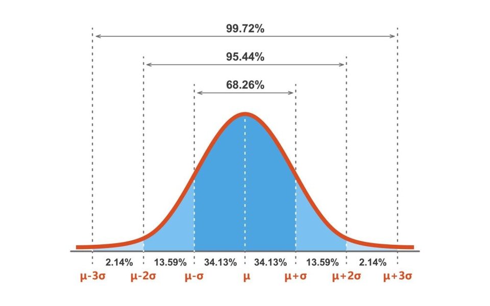
The image above depicts a typical normal distribution. The peak of the curve represents the mean (average) value, and the spread of the curve is determined by the standard deviation. In our light bulb scenario, the mean lifespan is 3000 hours, and the standard deviation is 400 hours. The curve shows that most bulbs will have a lifespan close to the mean, with fewer bulbs having lifespans far above or below it.

Key features of a normal distribution include:

Symmetry: The curve is symmetric around the mean.
Bell Shape: The curve has a bell shape, with the highest point at the mean.
Empirical Rule: Approximately 68% of the data falls within one standard deviation of the mean, 95% within two standard deviations, and 99.7% within three standard deviations.

Understanding the normal distribution helps us interpret probabilities and make predictions about the data. In the case of light bulbs, it allows us to estimate the likelihood of a bulb having a lifespan within a certain range.

Video Explanation: Objective vs. Subjective Probability

To further clarify the concepts of objective and subjective probability, the following video provides a concise explanation and real-world examples.

This video, titled "Objective & Subjective Probabilities | Independent & Mutually," offers a clear distinction between objective and subjective probabilities, along with discussions on independent and mutually exclusive events. From 0:14 to 3:42, the video specifically addresses the differences and applications of objective and subjective probability. The presenter elucidates how objective probability relies on factual data and empirical evidence, while subjective probability is rooted in personal beliefs and judgment. Real-world examples are provided to illustrate these concepts, making it easier to understand how each type of probability is used in different scenarios.

FAQ

What is the Z-score and why is it important?

The Z-score measures how many standard deviations an element is from the mean. It's important because it allows us to standardize any normal distribution, making it easier to calculate probabilities using a standard normal table.

How can probability theory be applied in everyday life?

Probability theory is used in various aspects of everyday life, including weather forecasting, sports analytics, insurance, finance, and medical decisions. It helps in quantifying uncertainty and making informed decisions.

What is the difference between a sample space and an event?

The sample space is the set of all possible outcomes of a random experiment, while an event is a subset of the sample space, representing a specific set of outcomes.

When should I use objective probability vs. subjective probability?

Use objective probability when there is sufficient historical data available. Use subjective probability when data is scarce, or when dealing with unique, non-repeatable events where personal judgment is necessary.

Can subjective probability be useful in business?

Yes, subjective probability can be useful in business forecasting, especially when assessing the likelihood of success for new products or strategies where historical data is limited.

References

Last updated April 11, 2025