Unveiling the Odds: Light Bulb Lifespans and the Power of Probability

Exploring how probability helps predict product life, manage uncertainty, and distinguish between data-driven facts and personal beliefs.

Highlights

Calculating Lifespan Probability: The likelihood of a specific light bulb lasting less than 2000 hours, given a mean life of 3000 hours and a standard deviation of 400 hours, is very low (approximately 0.62%).
Probability Theory's Reach: This mathematical framework is crucial for navigating uncertainty in fields ranging from engineering and finance to medicine and everyday decision-making.
Objective vs. Subjective Probability: Understanding the difference between probability based on verifiable data (objective) and probability based on personal judgment (subjective) is key to critical evaluation.

a) Calculating the Probability of Early Failure

You've asked about the probability of a randomly selected light bulb having a lifespan of less than 2000 hours, given that the manufacturer's bulbs have an average (mean) life of 3000 hours and a standard deviation of 400 hours. Since the lifespans are described as following a normal distribution (a common pattern for such measurements), we can use statistical methods to calculate this probability.

Understanding Normal Distribution

A normal distribution, often visualized as a bell curve, shows that most values cluster around the mean, with values becoming less frequent the further they are from the mean. The standard deviation measures the spread or dispersion of the data around the mean.

The Z-Score Calculation

To find the probability for a specific value (2000 hours) within this distribution, we first calculate the Z-score. The Z-score tells us how many standard deviations a particular value is away from the mean.

The formula for the Z-score is:

\[ Z = \frac{X - \mu}{\sigma} \]

Where:

\( X \) = The specific value of interest (2000 hours)
\( \mu \) = The mean lifespan (3000 hours)
\( \sigma \) = The standard deviation (400 hours)

Plugging in the values:

\[ Z = \frac{2000 - 3000}{400} = \frac{-1000}{400} = -2.5 \]

This Z-score of -2.5 means that a lifespan of 2000 hours is 2.5 standard deviations *below* the mean lifespan of 3000 hours.

Finding the Probability

Next, we use the Z-score to find the corresponding probability from a standard normal distribution table (also known as a Z-table) or a calculator. This table gives the cumulative probability, which is the probability of a value being less than or equal to the Z-score.

For \( Z = -2.5 \), the cumulative probability is approximately 0.0062.

Therefore, the probability that a randomly selected bulb will have a life of less than 2000 hours is approximately 0.0062, or 0.62%. This is a very small probability, indicating that it's quite rare for one of these bulbs to fail so early, based on the manufacturer's data.

b) When Do We Need Probability Theory?

Probability theory isn't just for mathematicians; it's a fundamental tool for understanding and quantifying uncertainty in countless real-world situations. We need it whenever we deal with randomness, incomplete information, or the need to predict the likelihood of future events.

Key Application Areas:

Risk Assessment & Management: In finance, insurance, and project management, probability helps evaluate the chances of losses, accidents, or failures, enabling informed decisions about mitigation strategies (e.g., setting insurance premiums, diversifying investments).
Science and Research: From quantum mechanics to genetics and epidemiology, probability models help analyze experimental data, test hypotheses, and understand natural phenomena (e.g., predicting disease spread, determining the significance of clinical trial results).
Engineering and Quality Control: Engineers use probability to assess the reliability and lifespan of components (like the light bulbs in our example), design robust systems, and implement quality control measures to minimize defects.
Machine Learning and Data Science: Probabilistic models are the backbone of many machine learning algorithms used for prediction, classification, and pattern recognition (e.g., spam filters, recommendation systems).
Decision Making (Everyday & Business): From deciding whether to bring an umbrella based on the weather forecast (a probabilistic prediction) to businesses forecasting sales or planning inventory, probability helps weigh potential outcomes.
Games and Gambling: Probability governs the odds in games of chance, from lotteries to card games.

In essence, probability theory provides a mathematical framework to reason about uncertainty, make predictions, and make better decisions when outcomes are not guaranteed.

Visualizing Probability's Reach

This mind map illustrates the diverse fields where probability theory plays a critical role:

mindmap root["Probability Theory Applications"] ["Science & Research"] ["Epidemiology (Disease Spread)"] ["Genetics (Inheritance Patterns)"] ["Physics (Quantum Mechanics)"] ["Clinical Trials (Treatment Efficacy)"] ["Engineering"] ["Quality Control (Defect Rates)"] ["Reliability Analysis (Lifespan Prediction)"] ["System Design (Failure Analysis)"] ["Finance & Economics"] ["Investment Analysis (Stock Prediction)"] ["Insurance (Risk & Premiums)"] ["Economic Forecasting"] ["Technology"] ["Machine Learning (Predictions)"] ["Computer Science (Algorithms)"] ["Network Analysis (Traffic Flow)"] ["Everyday Life"] ["Weather Forecasting"] ["Games of Chance"] ["Personal Risk Assessment"] ["Medicine"] ["Diagnosis (Likelihood of Disease)"] ["Treatment Outcomes"]

c) Core Concepts: Sample Space, Sample Points, and Events

To work with probability systematically, we use a few fundamental concepts that define the structure of a random experiment or situation.

Sample Space (S)

The sample space is the collection or set of *all possible distinct outcomes* of a random experiment. It represents the entire universe of possibilities for that specific experiment.

Example (Coin Toss): If you toss a single coin, the sample space is \( S = \{ \text{Heads, Tails} \} \).
Example (Dice Roll): If you roll a standard six-sided die, the sample space is \( S = \{ 1, 2, 3, 4, 5, 6 \} \).
Example (Light Bulb): For the light bulb lifespan experiment, the sample space is theoretically all possible non-negative durations the bulb could last, often represented as \( S = [0, \infty) \) hours, although practically limited by observed maximums.

The sample space must be exhaustive (include all possibilities) and the outcomes within it should be mutually exclusive (only one outcome can occur per trial).

Sample Points

A sample point is simply a *single possible outcome* within the sample space. It's one specific result of the random experiment. Each element listed in the sample space set is a sample point.

Example (Coin Toss): "Heads" is a sample point. "Tails" is another sample point.
Example (Dice Roll): The number "4" is a sample point. The number "1" is another sample point.
Example (Light Bulb): A specific lifespan, like "2850.5 hours", is a sample point within the continuous sample space.

Events (E)

An event is a *subset* of the sample space. It consists of one or more sample points that share a specific characteristic or meet a certain condition. We often want to calculate the probability of specific events occurring.

Example (Dice Roll):
- The event "rolling an even number" corresponds to the subset \( E_{\text{even}} = \{ 2, 4, 6 \} \).
- The event "rolling a number greater than 4" corresponds to the subset \( E_{>4} = \{ 5, 6 \} \).
- The event "rolling a 3" is a simple event corresponding to the subset \( E_{3} = \{ 3 \} \).
Example (Light Bulb):
- The event "the bulb lasts less than 2000 hours" (which we calculated in part a) corresponds to the subset of all sample points (lifespans) between 0 and 1999.99... hours.
- The event "the bulb lasts longer than the mean life" corresponds to the subset of all lifespans greater than 3000 hours.

Understanding these concepts allows us to precisely define the outcomes and conditions we are interested in when analyzing random phenomena.

d) Objective vs. Subjective Probability: Data vs. Belief

Probability quantifies likelihood, but how that likelihood is determined can differ. The main distinction lies between objective and subjective probability.

Objective Probability

Basis: Based on observable phenomena, historical data, frequency of past events, or logical/mathematical models where outcomes are equally likely (like a fair coin toss).
Determination: Calculated using empirical evidence, experiments, or mathematical formulas based on the physical properties or established patterns of the system.
Characteristics: Considered factual, verifiable, repeatable, and generally agreed upon given the same data or model. It's independent of personal opinions.
Example: The probability of drawing an Ace from a standard 52-card deck is 4/52 = 1/13. This is based on the fixed composition of the deck. The probability calculated for the light bulb (0.0062) is objective because it's derived from the given mean and standard deviation, assumed to be based on collected manufacturing data.

Subjective Probability

Basis: Based on personal judgment, intuition, experience, feelings, or beliefs. It reflects an individual's degree of confidence in an outcome occurring.
Determination: Assigned by an individual based on their personal assessment of the situation, which may incorporate some data but is heavily influenced by personal interpretation.
Characteristics: Personal, varies between individuals, not directly verifiable through frequency or experiment, can be influenced by biases.
Example: A sports fan estimating the probability of their team winning the next match based on their "gut feeling". An entrepreneur estimating the probability of a new business venture succeeding based on their personal market insights and optimism, without extensive historical data.

Comparing the Two Approaches

While objective probability is preferred in scientific and rigorous statistical analysis due to its basis in evidence, subjective probability plays a role in situations with limited data or unique events where past frequencies aren't available or applicable. Bayesian statistics often incorporates subjective prior beliefs which are then updated with objective data. This radar chart visually contrasts the typical characteristics:

Summary Table: Objective vs. Subjective Probability

This table provides a concise comparison:

Feature	Objective Probability	Subjective Probability
Basis	Historical data, frequencies, logical analysis, experiments	Personal judgment, beliefs, intuition, experience
Determination	Mathematical calculation, empirical observation	Personal assessment, degree of confidence
Consistency	High - Generally consistent across different observers given the same data/model	Low - Varies significantly between individuals
Verifiability	Can often be verified through repeated trials or checking against data	Difficult or impossible to verify empirically
Example	Probability of rolling a 6 on a fair die (1/6); Lifespan probability based on manufacturer data	Estimating the chance of rain based on how the sky looks; Predicting election results based on personal opinion
Primary Use	Scientific research, engineering, statistics, games of chance	Personal decision-making, situations with no historical data, Bayesian inference (as priors)

Visualizing Light Bulb Production and Testing

The calculation regarding light bulb lifespan connects directly to manufacturing processes and quality control. Manufacturers perform extensive testing to determine metrics like the mean lifespan and standard deviation. These images provide context on how light bulbs are made and tested.

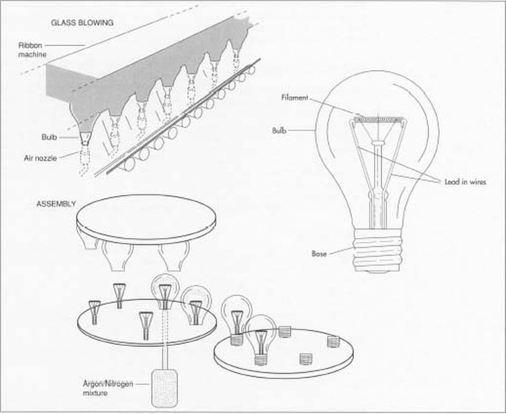
Illustration of steps in light bulb manufacturing.

Historical image of light bulb life test racks, used to gather lifespan data.

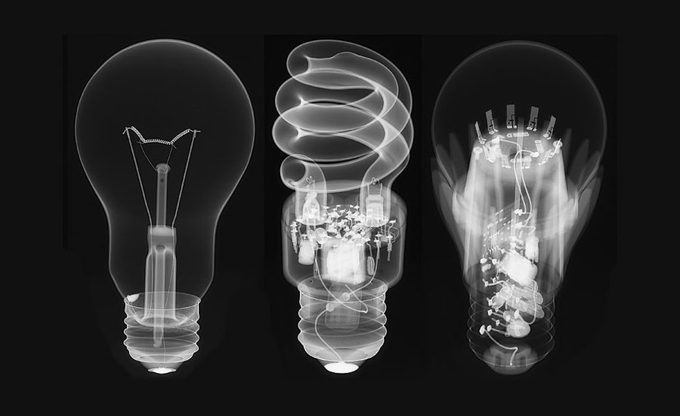
Modern quality control techniques, like X-ray tomography, ensure product integrity, indirectly relating to lifespan reliability.

Gathering data through such testing allows manufacturers to establish the normal distribution parameters (mean and standard deviation) used in probability calculations like the one performed earlier.

Calculating Probabilities with Normal Distribution

The calculation performed for the light bulb lifespan relies heavily on understanding the normal distribution and how to use Z-scores. This video provides a visual explanation of how to find probabilities related to normally distributed data using Z-tables, similar to the steps taken for the light bulb problem.

Watching this can help solidify the process of converting a real-world value (like 2000 hours) into a Z-score and then finding the corresponding area (probability) under the standard normal curve.

Frequently Asked Questions (FAQ)

What is a normal distribution (bell curve)?

A normal distribution is a continuous probability distribution characterized by its symmetrical, bell-shaped curve. Key features include:

The highest point of the curve is at the mean (average), which is also the median (middle value) and mode (most frequent value).
The curve is symmetrical around the mean.
The total area under the curve equals 1 (or 100%), representing the total probability of all possible outcomes.
The spread of the curve is determined by the standard deviation. A smaller standard deviation means the data points are clustered closer to the mean (taller, narrower curve), while a larger standard deviation means the data is more spread out (shorter, wider curve).

Many natural phenomena and measurements, like human height, measurement errors, and, in this case, the lifespan of manufactured components like light bulbs, tend to follow a normal distribution.

Why do we use Z-scores?

Z-scores are used to standardize values from different normal distributions, allowing us to compare them and calculate probabilities using a single reference: the standard normal distribution.

Standardization: The standard normal distribution has a mean of 0 and a standard deviation of 1. Converting a value (like the 2000-hour lifespan) to a Z-score transforms it into its equivalent position on this standard scale.
Comparison: Z-scores allow comparison of values from distributions with different means and standard deviations. For example, you could compare how unusual a 2000-hour lifespan is for this bulb type versus how unusual a different lifespan is for another bulb type with different parameters.
Probability Calculation: Standard normal distribution tables (Z-tables) or statistical software provide the cumulative probabilities associated with Z-scores. By converting our value (2000 hours) to a Z-score (-2.5), we could easily look up the probability P(Z < -2.5).

Essentially, Z-scores act as a universal language for normal distributions.

Can subjective probability be useful?

Yes, subjective probability can be very useful, especially in situations where objective data is scarce, unreliable, or non-existent. Examples include:

Novel Situations: Assessing the likelihood of success for a completely new product launch or a unique research project where no historical precedent exists.
Personal Decisions: Making choices based on personal risk tolerance and beliefs, like deciding on a career change or making a specific investment based on expert opinion (which is often subjective).
Bayesian Statistics: Subjective probabilities often serve as initial "prior beliefs" in Bayesian analysis. These priors are then formally updated with objective data as it becomes available, leading to more refined "posterior probabilities". This combines personal judgment with empirical evidence.

While it lacks the rigor of objective probability and is prone to bias, subjective probability provides a way to quantify belief and make decisions under extreme uncertainty. It's crucial, however, to be aware of its limitations and potential biases.