Estimating a Quantile Regression Model with Threshold Using Genetic Algorithms

A Comprehensive Guide to Enhancing Predictive Models with Advanced Optimization Techniques

Key Takeaways

Integration of Genetic Algorithms: Genetic algorithms optimize threshold parameters, enhancing model flexibility and accuracy.
Robustness and Flexibility: Quantile regression with threshold effects handles nonlinear relationships and is resilient to outliers.
Comprehensive Implementation Steps: From model specification to validation, a structured approach ensures robust estimates.

Introduction to Quantile Regression with Thresholds

Quantile regression extends traditional regression analysis by estimating conditional quantiles of the response variable, providing a more comprehensive view of the relationship between variables. Incorporating a threshold into a quantile regression model allows for modeling different regimes or regimes switching behavior based on a threshold variable. This approach is particularly useful in scenarios where the relationship between predictors and the response variable changes once the threshold is surpassed.

Conceptual Framework

Quantile Regression Explained

Unlike ordinary least squares (OLS) regression, which estimates the mean of the dependent variable conditional on the predictors, quantile regression targets specific quantiles (e.g., median, quartiles). This allows for a more nuanced understanding of the data distribution and is especially beneficial when the data exhibit heteroscedasticity or non-normal error distributions.

Threshold Effects in Regression Models

Introducing a threshold in a regression model accounts for changes in the relationship between the predictors and the response variable once a certain value of a threshold variable is crossed. This is essential for capturing potential regime shifts or non-linear dynamics within the data.

Genetic Algorithms as Optimization Tools

Genetic algorithms (GAs) are heuristic search methods inspired by the process of natural selection. They are particularly effective for optimizing complex, non-linear, and multi-modal functions where traditional optimization techniques may falter. In the context of quantile regression with thresholds, GAs can optimize the threshold parameter and regression coefficients simultaneously.

Integrating Genetic Algorithms with Quantile Regression

Model Specification

The quantile regression model with a threshold can be specified as follows:

Model Structure:

y = Xβ₁ if z ≤ γ y = Xβ₂ if z > γ

Here:

y is the response variable.
X is the matrix of predictors.
β₁ and β₂ are the regression coefficients for the respective regimes.
z is the threshold variable.
γ is the unknown threshold parameter.

Optimization with Genetic Algorithms

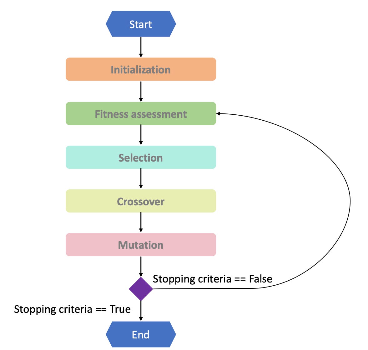
Genetic algorithms are employed to find the optimal values of the threshold parameter (γ) and the regression coefficients (β₁ and β₂) by minimizing the quantile loss function. The process involves encoding these parameters into a chromosome, defining a fitness function based on the quantile loss, and evolving the population of solutions through selection, crossover, and mutation.

Steps in the Genetic Algorithm

Initialization: Generate an initial population of potential solutions, each representing a set of parameters (β₁, β₂, γ).
Fitness Evaluation: Calculate the fitness of each solution based on how well it minimizes the quantile loss function.
Selection: Select the fittest solutions to serve as parents for the next generation.
Crossover: Combine pairs of parents to produce offspring, inheriting traits from both.
Mutation: Introduce random changes to some offspring to maintain diversity within the population.
Iteration: Repeat the evaluation, selection, crossover, and mutation processes for multiple generations until convergence.

Implementation Steps

1. Define the Quantile Loss Function

The quantile loss function, also known as the "check function," is defined as:

Check Function:
ρτ(u) = u(τ – I(u < 0))

Where:

u is the residual (difference between observed and predicted values).
τ is the target quantile (e.g., 0.5 for median).
I(u < 0) is an indicator function that equals 1 if u < 0 and 0 otherwise.

2. Initialize the Genetic Algorithm

Start by creating an initial population of possible threshold values and regression coefficients. Each member of the population is represented as a chromosome containing values for β₁, β₂, and γ.

3. Define the Fitness Function

The fitness function assesses how well a particular set of parameters minimizes the quantile loss. Since genetic algorithms typically maximize the fitness value, the quantile loss is negated to convert the minimization problem into a maximization one.

4. Configure Genetic Algorithm Parameters

Key parameters include:

Population Size: Number of chromosomes in each generation.
Number of Generations: How many iterations the algorithm will run.
Crossover Rate: Probability of combining two chromosomes to produce offspring.
Mutation Rate: Probability of randomly altering gene values to introduce variability.

5. Run the Genetic Algorithm

Execute the genetic algorithm, allowing it to evolve the population over multiple generations. The algorithm seeks to find the combination of parameters that yields the highest fitness score, indicating the best fit according to the quantile loss function.

6. Retrieve and Validate the Best Solution

Once the algorithm converges, extract the best-performing set of parameters. Validate the model using separate validation data to ensure robustness and generalizability of the estimated threshold and regression coefficients.

Practical Implementation: Python Example

Sample Python Code Using PyGAD

Below is an example of how to implement a quantile regression model with a threshold using the PyGAD library in Python. This example simulates data, defines the quantile loss function, and configures and runs the genetic algorithm to estimate the model parameters.

#---------------------------
# Step 1. Import libraries
import numpy as np
import pygad

#---------------------------
# Step 2. Define the check loss function for quantile regression
def check_loss(residuals, tau):
    # residuals: vector of differences
    # tau: target quantile (e.g., 0.5 for median)
    return np.sum((tau - (residuals < 0)) * residuals)

#---------------------------
# Step 3. Define the fitness function to be maximized by GA
# (we convert our minimization problem into maximization by taking a negative)
def fitness_func(solution, solution_idx):
    # Assume solution structure: first p parameters for beta1, next p for beta2, last is gamma
    p = X.shape[1]
    beta1 = solution[0:p]
    beta2 = solution[p:2*p]
    gamma = solution[-1]
    
    # Compute predictions and residuals
    predictions = np.empty_like(y)
    for i in range(len(y)):
        if z[i] <= gamma:
            predictions[i] = np.dot(X[i], beta1)
        else:
            predictions[i] = np.dot(X[i], beta2)
    
    residuals = y - predictions
    loss = check_loss(residuals, tau)
    
    # GA maximizes fitness, so we use negative loss.
    fitness = -loss
    return fitness

#---------------------------
# Step 4. Create simulated (or load your) data
# For example, let’s simulate some data.
np.random.seed(123)
n = 100
p = 2  # number of predictors

X = np.random.normal(0, 1, (n, p))
# Let the threshold variable be the first column of X, or a separate variable:
z = X[:, 0]
true_gamma = 0.0
true_beta1 = np.array([1.5, -2.0])
true_beta2 = np.array([0.5, 1.0])
noise = np.random.normal(0, 1, n)

y = np.zeros(n)
for i in range(n):
    if z[i] <= true_gamma:
        y[i] = np.dot(X[i], true_beta1) + noise[i]
    else:
        y[i] = np.dot(X[i], true_beta2) + noise[i]

# Set the quantile of interest
tau = 0.5  # median regression, for instance

#---------------------------
# Step 5. Configure the GA.
# Define lower and upper bounds for each parameter.
# Here we assume β's in e.g. [-5, 5] and gamma in [min(z), max(z)].
gene_space = []
for i in range(2*p):
    gene_space.append({'low': -5, 'high': 5})
gene_space.append({'low': np.min(z), 'high': np.max(z)})

ga_instance = pygad.GA(num_generations=200,
                       num_parents_mating=10,
                       fitness_func=fitness_func,
                       sol_per_pop=50,
                       num_genes=2*p+1,
                       gene_space=gene_space,
                       mutation_percent_genes=10,
                       mutation_type="random",
                       stop_criteria=["reach_0"])  # You can adjust stop criteria

#---------------------------
# Step 6. Run the GA.
ga_instance.run()

#---------------------------
# Step 7. Retrieve the best solution.
solution, solution_fitness, solution_idx = ga_instance.best_solution()
print("Best solution parameters (β1, β2, γ):")
print(solution)
print("Fitness (negative loss):", solution_fitness)

# For further analysis, you might want to compute the loss and compare with other estimators.

Explanation of the Code

Step 1: Import necessary libraries, including NumPy for numerical operations and PyGAD for implementing the genetic algorithm.

Step 2: Define the quantile check loss function, which penalizes residuals asymmetrically based on the target quantile.

Step 3: Create a fitness function that the genetic algorithm will maximize. This function computes the negative quantile loss for a given set of parameters.

Step 4: Simulate data that includes a threshold effect. The response variable y changes its relationship with predictors X based on the threshold variable z.

Step 5: Configure the genetic algorithm by defining the search space for each gene (parameters β₁, β₂, and γ) and setting GA parameters such as population size and number of generations.

Step 6: Run the genetic algorithm to evolve the population towards optimal solutions.

Step 7: Retrieve and display the best solution found by the GA, including the estimated regression coefficients and threshold value.

Considerations and Best Practices

Population Size and Generations: Larger populations and more generations increase the likelihood of finding a global optimum but require more computational resources.
Mutation Rate: Balancing mutation ensures diversity within the population, preventing premature convergence to local optima.
Parameter Scaling: Standardizing predictors can improve the performance of the genetic algorithm.
Multiple Runs: Running the GA multiple times can help verify the stability and robustness of the estimated parameters.

Advantages and Challenges

Advantages

Robustness to Outliers: Quantile regression inherently reduces the influence of outliers compared to mean regression.
Flexibility: The model can capture complex, non-linear relationships by allowing different regression coefficients across regimes.
Comprehensive Insights: Provides a detailed view of the impact of predictors across the entire distribution of the response variable.
Optimization Efficiency: Genetic algorithms effectively explore the parameter space, especially when dealing with multiple local minima.

Challenges

Computational Intensity: Genetic algorithms can be computationally demanding, especially with large datasets or complex models.
Parameter Tuning: Selecting appropriate GA parameters (e.g., population size, mutation rate) requires experimentation and expertise.
Local Optima: Despite their robustness, GAs may still converge to local optima if not properly configured.
Scalability: Scaling the model to handle high-dimensional data may introduce additional complexities.

Validation and Model Assessment

Cross-Validation Techniques

Implement cross-validation to assess the model's performance and generalizability. Techniques such as k-fold cross-validation can help evaluate how well the model predicts unseen data.

Performance Metrics

Use appropriate metrics to evaluate the model's performance:

Quantile Loss: Measures how well the model predicts the specified quantile.
Mean Absolute Error (MAE): Assesses the average magnitude of errors in the predictions.
Mean Squared Error (MSE): Penalizes larger errors more heavily than MAE.
R-squared: Indicates the proportion of variance explained by the model, although it is less commonly used in quantile regression.

Model Diagnostics

Conduct diagnostic checks to ensure the validity of the model:

Residual Analysis: Examining residuals can reveal patterns or heteroscedasticity not captured by the model.
Threshold Significance: Perform statistical tests to confirm the significance of the estimated threshold.
Stability Checks: Assess how sensitive the model is to changes in the data or parameter specifications.

Applications and Use Cases

Economics and Finance

Quantile regression with thresholds can model different market regimes, such as bull and bear markets, allowing for tailored investment strategies based on market conditions.

Environmental Studies

Analyzing environmental data with threshold effects can help identify critical points where environmental factors significantly influence outcomes, such as pollution levels exceeding safe limits.

Healthcare and Biostatistics

In clinical studies, thresholds can represent critical values of biomarkers, helping to differentiate between patient subgroups with distinct prognoses or treatment responses.

Conclusion

Estimating a quantile regression model with a threshold using genetic algorithms offers a powerful approach to capturing complex, non-linear relationships in data. By leveraging the optimization capabilities of genetic algorithms, researchers and practitioners can effectively identify threshold points and estimate regime-specific effects across different quantiles, providing deeper insights and more accurate predictive models. Despite the challenges related to computational demands and parameter tuning, the robustness and flexibility of this methodology make it a valuable tool in various domains, including economics, finance, environmental studies, and healthcare.

References

Last updated February 11, 2025