Handling Multi-Band Raster Data in Python

A Comprehensive Guide to Reading, Processing, and Visualizing Multi-Band Raster Files

Highlights

Library Ecosystem: Use Rasterio, GDAL, and NumPy for efficient multi-band raster reading, writing, and analysis.
Data Management: Techniques for stacking single-band files, spatial consistency, and memory management are essential.
Visualization & Analysis: Create RGB composites and perform spectral analysis while handling NoData and normalization issues.

Introduction

Multi-band raster data, which contains several layers representing different portions of the electromagnetic spectrum, is pivotal in remote sensing, environmental monitoring, and geospatial analysis. In Python, handling such data requires an array of specialized libraries that allow both processing and visualization. This guide explains methods to read, process, analyze, and visualize multi-band raster files using Python's robust geospatial ecosystem, which includes packages like Rasterio, GDAL, NumPy, and EarthPy.

Key Libraries and Tools

Python offers a variety of libraries designed to handle multi-band raster data. The most commonly employed include:

Rasterio

Rasterio is built on top of GDAL and provides a Pythonic interface to work with raster data. It simplifies the process of reading and writing raster files by abstracting complex GDAL operations. With Rasterio, multi-band rasters can be loaded directly into NumPy arrays, enabling seamless integration with other scientific libraries.

GDAL (Geospatial Data Abstraction Library)

GDAL is a foundational library in geospatial processing that supports a wide range of raster formats and operations. While its native interface is C/C++, Python bindings are available. GDAL is powerful for tasks like extracting bands, warping images, and performing re-projections. It also facilitates vector to raster conversions.

NumPy and EarthPy

NumPy provides a high-performance multidimensional array object, perfect for numerical computations on raster data. EarthPy further eases the stacking and plotting of raster images, particularly when compositing multiple bands into a single image.

Reading Multi-Band Raster Data

Reading multi-band raster data is the first step in many geospatial processing workflows. Both Rasterio and GDAL offer straightforward methods for accessing multi-band information.

Using Rasterio for Reading Data

Rasterio simplifies the process with its context manager and built-in methods:

Example Code

# Import necessary libraries
import rasterio
import numpy as np

# Open the multi-band raster file
with rasterio.open('multiband_image.tif') as src:
    # Read all bands as a 3D NumPy array with dimensions (bands, rows, columns)
    raster_data = src.read()
    
    # Optionally, read specific bands (e.g., first and second bands)
    band1 = src.read(1)
    band2 = src.read(2)
    
    # Print metadata to understand spatial details and data types
    print(src.meta)

In this example, the entire dataset is read into a NumPy array, enabling further numerical manipulation.

Using GDAL for Reading Data

GDAL allows more granular control through its dataset and band objects. The following snippet demonstrates how to access individual bands:

Example Code

# Import the GDAL module
from osgeo import gdal

# Open the multi-band raster dataset
dataset = gdal.Open('multiband_image.tif')

# Read a specific band (here, band number 1)
band1 = dataset.GetRasterBand(1).ReadAsArray()

# Loop through bands if needed
num_bands = dataset.RasterCount
for i in range(1, num_bands + 1):
    band_data = dataset.GetRasterBand(i).ReadAsArray()
    # Process each band_data as required

This method grants explicit control over the dataset and effective handling of multi-band arrays.

Stacking Raster Bands and Creating Multi-Band Rasters

When individual single-band files are available, they can be merged or “stacked” to form a multi-band raster dataset. This process involves ensuring that all bands share the same spatial extent, coordinate reference system (CRS), and resolution.

Using Rasterio to Stack Bands

Stacking multiple single-band files into a multi-band raster is simplified using Rasterio. The following code demonstrates how to combine single-band images:

Stacking Example Code

import rasterio
import glob

# List all single-band raster files
files = glob.glob('path/to/single_band_files/*.tif')

# Open one file to retrieve metadata and update the count
with rasterio.open(files[0]) as src0:
    meta = src0.meta
meta.update(count=len(files))

# Write the multi-band raster file
with rasterio.open('stacked_multiband.tif', 'w', **meta) as dst:
    for index, filename in enumerate(files, start=1):
        with rasterio.open(filename) as src:
            dst.write(src.read(1), index)

Using EarthPy for Stacking

EarthPy offers a helper function, stack(), to combine multiple raster files efficiently:

EarthPy Stacking Example

import earthpy as et

# Assuming you have a list of file paths for the single-band rasters
stacked_array = et.stack(['band1.tif', 'band2.tif', 'band3.tif'])

Visualization and Analysis of Multi-Band Rasters

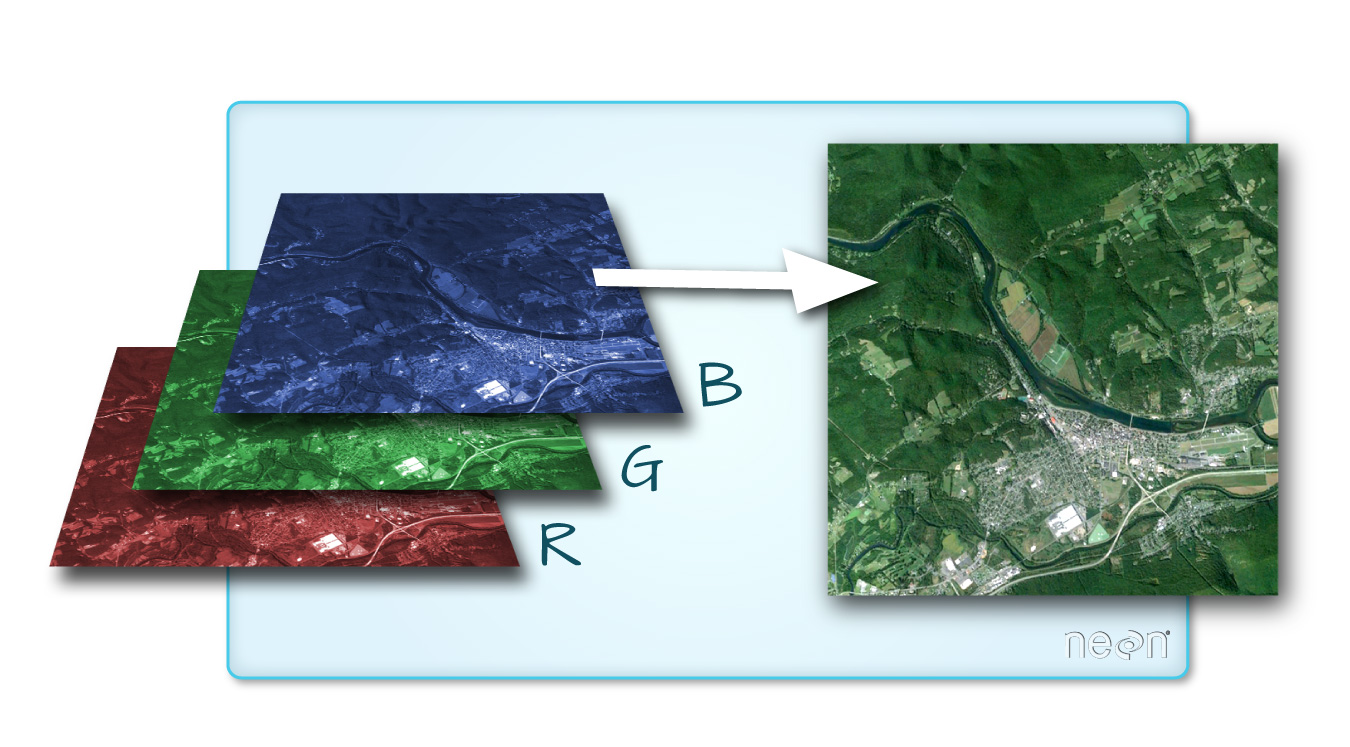
One critical application of multi-band raster data is the generation of RGB composites, which entails selecting appropriate bands to form a natural or false-color image. These composites help in easy interpretation of satellite imagery.

Creating RGB Composites

For example, a typical RGB composite for Landsat imagery may involve bands 4 (red), 3 (green), and 2 (blue). The following snippet demonstrates how to create and display an RGB composite using Rasterio and Matplotlib:

RGB Composite Code

import rasterio
import numpy as np
import matplotlib.pyplot as plt

# Open the Landsat multi-band file
with rasterio.open('landsat_image.tif') as src:
    # Read bands necessary for the RGB composite
    red = src.read(4)
    green = src.read(3)
    blue = src.read(2)

# Normalize the bands for proper display
def normalize(array):
    return (array - array.min()) / (array.max() - array.min())

red_norm = normalize(red)
green_norm = normalize(green)
blue_norm = normalize(blue)

# Stack bands and prepare for display (Note: order might be blue, green, red for display libraries)
rgb = np.dstack((red_norm, green_norm, blue_norm))

plt.imshow(rgb)
plt.title("RGB Composite Image")
plt.axis('off')
plt.show()

Normalization is critical for ensuring that the differences in range between bands do not skew the visual representation. Adjusting data values to a common range (usually 0 to 1) is a common pre-processing step.

Handling NoData Values and Band Reordering

Many raster datasets include NoData values that need special handling. These can be managed by masking the data or assigning distinct colors. It is also vital to ensure that the band order in your composite is correct. Some imagery sources store bands in reverse order, necessitating reordering before visualization.

Advanced Techniques in Multi-Band Raster Data Processing

Beyond the basics of input and output, advanced processing can significantly enhance the analysis quality. Techniques include pixel-level spectral analysis, statistical computation per band, and transformation operations.

Statistical Analysis and Array Manipulations

Once raster data is loaded into a NumPy array, you can perform various statistical operations such as calculating means, standard deviations, or even custom functions on a per-band basis. For example, calculating the mean across each band can be achieved with:

Statistical Analysis Example

import numpy as np

# Assume raster_data is structured as (bands, rows, columns)
band_means = np.mean(raster_data, axis=(1, 2))
print("Mean value for each band:", band_means)

This method helps in understanding the brightness and contrast levels across different spectral bands and aids in further processing or thresholding tasks.

Creating Custom Band Composites

Apart from standard RGB composites, custom composites can be created to highlight specific features such as vegetation, water bodies, or urban areas. For instance, a false-color composite might include bands such as near-infrared (NIR), red, and green, thereby emphasizing vegetation health.

Custom Composite Example

# Read the necessary bands for a false-color composite
with rasterio.open('multiband_image.tif') as src:
    nir = src.read(5)  # Near-infrared
    red = src.read(4)
    green = src.read(3)

# Normalize bands
nir_norm = normalize(nir)
red_norm = normalize(red)
green_norm = normalize(green)

# Stack them for a false-color composite (NIR, red, green)
false_color = np.dstack((nir_norm, red_norm, green_norm))

plt.imshow(false_color)
plt.title("False-Color Composite")
plt.axis('off')
plt.show()

Such composites are useful in environmental monitoring and land cover classification tasks.

Efficient Data Management and Large File Handling

When working with extensive datasets or high-resolution imagery, managing system memory effectively becomes crucial. Both GDAL and Rasterio facilitate reading data in chunks, which allows processing without fully loading entire datasets into memory.

Chunking and Block Processing

Many raster files are divided into blocks or tiles, enabling block-level processing. This not only optimizes memory usage but also speeds up processing time for large datasets.

Chunk Processing Illustration

Aspect	Description
Memory Management	Process images in smaller chunks to prevent memory overrun.
Speed	Proper chunking can reduce the time spent on disk I/O.
Scalability	Allows handling of datasets that are larger than available RAM.

With block processing, you can iterate over areas of the image, process, and then write results before moving to the next block.

Compression and Data Type Optimization

When writing multi-band raster files, choosing file formats such as GeoTIFF with compression options (e.g., LZW or DEFLATE) can significantly reduce file size. Additionally, selecting optimal data types that faithfully represent the data without excessive memory cost is vital.

Additional Operations: Rasterizing Vector Data

In some scenarios, converting vector data to a raster format (rasterization) is required. This involves burning vector attributes into a raster grid, which can then be combined with other raster layers to form a multi-band output.

Vector to Raster Conversion

The process usually involves:

Defining the spatial resolution and output extent based on a reference raster.
Burning vector attributes such as temperature, elevation, or classifications into individual raster bands.
Stacking the resultant single-band rasters into a multi-band dataset.

Rasterization Example Concept

from osgeo import gdal, ogr

def rasterize_vector(ref_raster, vector_file, attribute):
    # Open reference raster to collect geospatial info
    ref = gdal.Open(ref_raster)
    geo_transform = ref.GetGeoTransform()
    projection = ref.GetProjection()
    cols = ref.RasterXSize
    rows = ref.RasterYSize
    # Create temporary raster for burning vector attribute
    mem_drv = gdal.GetDriverByName('MEM')
    target_ds = mem_drv.Create('', cols, rows, 1, gdal.GDT_Float32)
    target_ds.SetGeoTransform(geo_transform)
    target_ds.SetProjection(projection)
    
    # Open vector file and perform rasterization
    vector_ds = ogr.Open(vector_file)
    gdal.RasterizeLayer(target_ds, [1], vector_ds.GetLayer(), options=["ATTRIBUTE=" + attribute])
    return target_ds

# Example usage
output_raster = rasterize_vector('ref.tif', 'data.shp', 'elevation')

Best Practices for Multi-Band Raster Data Processing

Summarizing the tips and practices:

Always ensure that the data you are processing shares a common spatial reference and resolution.
Normalize band values to handle varying ranges across different spectral bands.
Handle NoData values to avoid skewed statistical analyses.
Use chunk or block processing to manage large datasets efficiently.
Select file formats supporting compression to optimize storage and I/O performance.

Conclusion

In conclusion, handling multi-band raster data in Python involves an array of strategies ranging from basic file reading and visualization to advanced band stacking, statistical analysis, and vector rasterization. The integration of libraries such as Rasterio, GDAL, NumPy, and EarthPy provides a flexible and robust framework to address the diverse use cases of remote sensing and geospatial analysis. Whether working with satellite imagery from Landsat or custom multi-band datasets, these tools enable efficient data manipulation, accurate visualization through RGB or custom composites, and scalable processing for large datasets. By following best practices in managing spatial consistency, handling NoData values, and optimizing memory usage, you can ensure that your geospatial analysis workflows will be both efficient and effective.

Handling Multi-Band Raster Data in Python

A Comprehensive Guide to Reading, Processing, and Visualizing Multi-Band Raster Files

Highlights

Introduction

Key Libraries and Tools

Rasterio

GDAL (Geospatial Data Abstraction Library)

NumPy and EarthPy

Reading Multi-Band Raster Data

Using Rasterio for Reading Data

Example Code

Using GDAL for Reading Data

Example Code

Stacking Raster Bands and Creating Multi-Band Rasters

Using Rasterio to Stack Bands

Stacking Example Code

Using EarthPy for Stacking

EarthPy Stacking Example

Visualization and Analysis of Multi-Band Rasters

Creating RGB Composites

RGB Composite Code

Handling NoData Values and Band Reordering

Advanced Techniques in Multi-Band Raster Data Processing

Statistical Analysis and Array Manipulations

Statistical Analysis Example

Creating Custom Band Composites

Custom Composite Example

Efficient Data Management and Large File Handling

Chunking and Block Processing

Chunk Processing Illustration

Compression and Data Type Optimization

Additional Operations: Rasterizing Vector Data

Vector to Raster Conversion

Rasterization Example Concept

Best Practices for Multi-Band Raster Data Processing

Conclusion

References

Recommended