Ithy - Transforming Signals: The Fascinating Mathematics Behind Rectangular Self-Convolution

Key Insights into Rectangular Self-Convolution

Elegant Transformation: When a rectangular function is convolved with itself, it always results in a triangular-shaped function
Width Doubling Property: The resulting triangular function has exactly twice the width of the original rectangular pulse
Overlap Principle: The triangular shape emerges from the changing overlap area as one rectangular pulse slides across another identical pulse

Understanding the Rectangular Function

The rectangular function, often denoted as rect(t), is a fundamental building block in signal processing and mathematics. It's defined as having a constant value (typically 1) over a specific interval and zero elsewhere:

For the standard rectangular function:

\[ \text{rect}(t) = \begin{cases} 1, & \text{if } |t| \leq \frac{1}{2} \ 0, & \text{if } |t| > \frac{1}{2} \end{cases} \]

This creates a "pulse" or "window" that is often used as a basic signal element. In many practical applications, we might use a more general representation where the rectangular function has width T and amplitude A:

\[ f(t) = \begin{cases} A, & \text{if } a \leq t \leq b \quad \text{(where } b-a=T\text{)} \ 0, & \text{otherwise} \end{cases} \]

What is Convolution?

Convolution is a mathematical operation that combines two functions to produce a third function expressing how the shape of one is modified by the other. For continuous functions, convolution is defined as:

\[ (f * g)(t) = \int_{-\infty}^{\infty} f(\tau) \cdot g(t-\tau) \, d\tau \]

In the specific case of self-convolution, we convolve a function with itself:

\[ (f * f)(t) = \int_{-\infty}^{\infty} f(\tau) \cdot f(t-\tau) \, d\tau \]

Self-Convolution of a Rectangular Function: The Mathematical Process

Step-by-Step Derivation

Let's consider a rectangular function f(t) with width T and height 1. The self-convolution is:

\[ (f * f)(t) = \int_{-\infty}^{\infty} f(\tau) \cdot f(t-\tau) \, d\tau \]

Since f(τ) is non-zero only when τ is within the rectangular pulse, and similarly, f(t-τ) is non-zero only when (t-τ) is within the pulse, the integral reduces to calculating the overlap between these two conditions.

Evaluating the Integral

For clarity, let's use a rectangular function defined on [0,T]:

\[ f(t) = \begin{cases} 1, & \text{if } 0 \leq t \leq T \ 0, & \text{otherwise} \end{cases} \]

The integral becomes:

\[ (f * f)(t) = \int_{-\infty}^{\infty} f(\tau) \cdot f(t-\tau) \, d\tau = \int_{0}^{T} f(t-\tau) \, d\tau \]

Now, f(t-τ) equals 1 only when 0 ≤ t-τ ≤ T, which gives us τ ≤ t ≤ τ+T. This creates three distinct cases:

Case 1 (t < 0): No overlap occurs, resulting in (f * f)(t) = 0
Case 2 (0 ≤ t ≤ T): Partial overlap occurs, giving (f * f)(t) = t
Case 3 (T < t ≤ 2T): Decreasing overlap occurs, giving (f * f)(t) = 2T-t
Case 4 (t > 2T): No overlap occurs, resulting in (f * f)(t) = 0

These four cases together form a triangular function with base width 2T and height T (or A²T if the original rectangle has amplitude A).

The Intuitive Explanation: Sliding Rectangles

Imagine sliding one rectangular pulse across another identical pulse. The convolution at each point represents the overlap area between these two pulses:

Initially, there's no overlap (result is zero)
As one pulse starts to overlap the other, the overlap area increases linearly
Maximum overlap occurs when the pulses are perfectly aligned
As the pulse continues sliding, the overlap decreases linearly
Eventually, no overlap remains (result returns to zero)

This process naturally creates a triangular shape, demonstrating why the self-convolution of a rectangular function always yields a triangular function.

Visual Representation of the Process

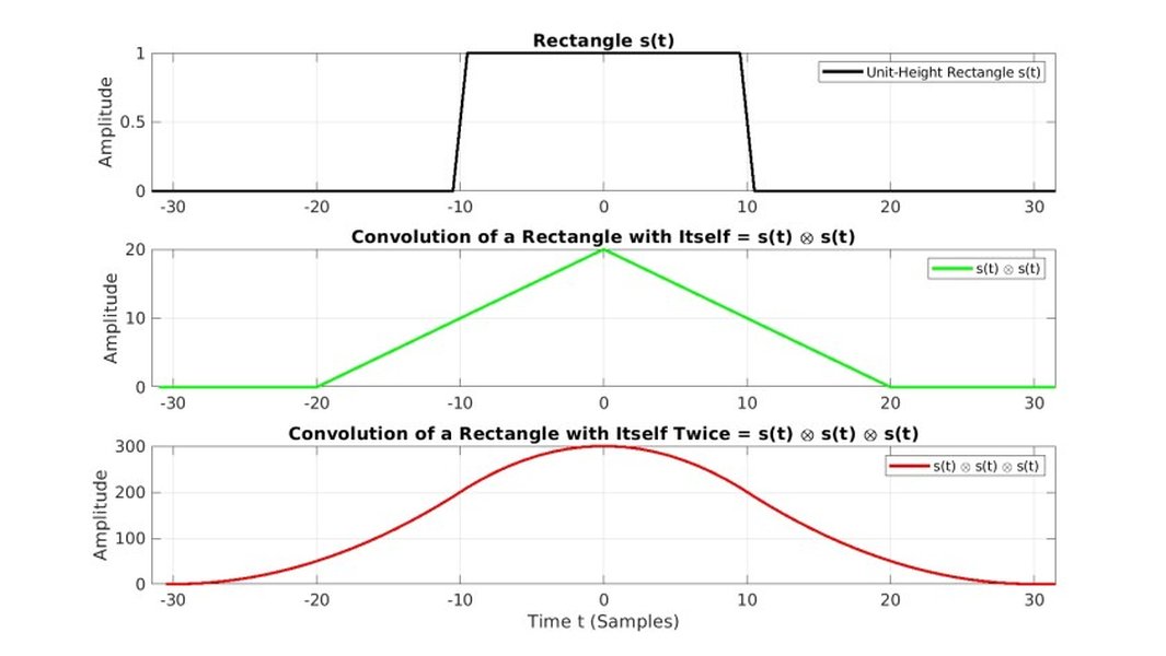
Visual representation of rectangular function convolution

Visualization of the convolution process showing how rectangular pulses create triangular results

Applications and Significance

The self-convolution of rectangular functions has numerous practical applications across various scientific and engineering disciplines:

Signal Processing Applications

Pulse Shaping: Used to shape rectangular pulses into smoother triangular pulses, reducing bandwidth requirements
Filter Design: Triangular filters can be implemented by convolving rectangular filters
System Analysis: Understanding how systems respond to rectangular inputs through convolution
Spectral Analysis: The spectrum of a rectangular pulse has periodic nulls related to sinc functions

Optics and Photonics

Triangular Pulse Generation: Photonic approaches utilize self-convolution of rectangular pulses
Diffraction Patterns: Describing light patterns through rectangular apertures
Optical Filter Design: Creating specific optical response profiles

Mathematical Properties

Central Limit Theorem: Multiple convolutions of rectangular functions approach a Gaussian distribution
Fourier Transform Relationships: The Fourier transform of a rectangular pulse is a sinc function
Convolution Theorem: Multiplication in frequency domain equals convolution in time domain

Comparison of Properties

Property	Rectangular Function	Self-Convoluted Result (Triangle)
Shape	Flat top with vertical edges	Peaked with linear slopes
Width	T	2T
Maximum Value	A	A²T (or T if A=1)
Continuity	Discontinuous at edges	Continuous everywhere
Differentiability	Non-differentiable at edges	Non-differentiable only at peak and ends
Fourier Transform	sinc function	sinc² function

Visual Analysis of Rectangular Self-Convolution

Radar Chart: Properties and Applications

The following radar chart illustrates the relative significance of various aspects of rectangular self-convolution across different domains:

Interactive Visual Demonstration

This video provides an excellent visual explanation of how the convolution of rectangular pulses works:

Concept Map: Self-Convolution of Rectangular Functions

This mindmap illustrates the key concepts, properties, and applications of rectangular self-convolution:

mindmap root["Self-Convolution of Rectangular Function"] ["Mathematical Process"] ["Definition"] ["Rectangular Function"] ["Convolution Integral"] ["Calculation"] ["Overlap Analysis"] ["Piecewise Integration"] ["Resulting Triangular Function"] ["Width = 2× Original"] ["Linear Rise and Fall"] ["Continuous Function"] ["Peak Value = T (for unit amplitude)"] ["Interpretation"] ["Sliding Overlap Area"] ["Time-Domain Effects"] ["Frequency-Domain Effects"] ["Applications"] ["Signal Processing"] ["Pulse Shaping"] ["Filter Design"] ["Optics"] ["Diffraction Patterns"] ["Triangular Pulse Generation"] ["Communications"] ["Bandwidth Management"] ["Multipath Channels"] ["Statistical Analysis"] ["Probability Density Functions"] ["Central Limit Theorem"]

Frequently Asked Questions

Why does the self-convolution of a rectangular function always result in a triangular function?

What happens if you convolve a rectangular function with itself multiple times?

How does the Fourier transform relate to the self-convolution of rectangular functions?

What are the practical advantages of triangular pulses over rectangular pulses in signal processing?

What happens when rectangular pulses of different widths are convolved?

Transforming Signals: The Fascinating Mathematics Behind Rectangular Self-Convolution

Discover how a simple rectangular pulse transforms into a triangular shape through self-convolution, revealing fundamental principles in signal processing