Navigating the Labyrinth: How Do SLAM's Filtering and Smoothing Algorithms Differ in Mapping Reality?

Unraveling the core distinctions between real-time estimation and comprehensive trajectory optimization in robotic mapping and localization.

Simultaneous Localization and Mapping (SLAM) is a cornerstone technology enabling autonomous systems, from robotic vacuum cleaners to self-driving cars, to understand and navigate their surroundings. At the heart of SLAM are algorithms that estimate the system's pose (position and orientation) and construct a map of the environment. These algorithms predominantly fall into two categories: filtering-based and smoothing-based approaches. Understanding their differences is crucial for selecting the appropriate method for a given application. This exploration delves into a detailed comparison, drawing upon scientific insights to illuminate their respective methodologies, strengths, and weaknesses.

Key Distinctions at a Glance

Filtering SLAM: Prioritizes real-time current state estimation using only the most recent sensor measurements and motion data. It's an incremental, online process.
Smoothing SLAM: Aims for global consistency by optimizing the entire trajectory and map simultaneously, considering all or a large batch of past measurements. This is often an offline or less frequent, more computationally intensive process.
Application Suitability: The choice hinges on specific needs—filtering excels in speed and resource-constrained scenarios, while smoothing is favored for higher accuracy and offline analysis where global map consistency is paramount.

Foundational Principles: Filtering vs. Smoothing

Both filtering and smoothing approaches in SLAM aim to solve the complex problem of a robot building a map while simultaneously determining its location within that map. However, they tackle this challenge with fundamentally different mathematical and computational strategies.

A conceptual overview of the SLAM process, where a robot simultaneously maps its environment and localizes itself.

Filtering-Based SLAM: The Incremental Estimator

Filtering-based SLAM treats the problem as a recursive state-estimation task. It focuses on estimating the current state of the robot (pose) and the map features using the most recent measurements. This approach is inherently online, processing data sequentially as it arrives.

Core Mechanism

Filters, like the Extended Kalman Filter (EKF), Unscented Kalman Filter (UKF), or Particle Filters, operate in a predict-update cycle:

Prediction: The robot's next state is predicted based on its motion model.
Update: When new sensor measurements (e.g., observing landmarks) are received, the state estimate and its uncertainty (covariance) are updated.

Older measurements are typically summarized or implicitly incorporated into the current state estimate and then effectively discarded to manage computational load. The EKF-SLAM, for instance, linearizes non-linear motion and observation models and maintains a Gaussian belief over the current state and landmark positions.

Key Characteristics

Maintains an estimate of the current robot pose and map.
Processes data incrementally and in real-time.
Computationally efficient for each update step.
Examples: EKF-SLAM, UKF-SLAM, FastSLAM (which uses particle filters).

Smoothing-Based SLAM: The Global Optimizer

Smoothing-based SLAM, also known as batch SLAM or full SLAM, takes a more holistic view. It considers all (or a significant window of) past measurements and robot poses to estimate the entire trajectory of the robot and the map simultaneously. This is typically formulated as a large-scale optimization problem.

Core Mechanism

Smoothing methods aim to find the set of robot poses and landmark positions that best explain all observed data. This is often framed as a Maximum A Posteriori (MAP) estimation problem and visualized as a factor graph or pose graph:

Graph Construction: Robot poses and landmark positions are nodes in a graph. Constraints derived from motion models (odometry) and sensor measurements (observations of landmarks or loop closures) form the edges.
Optimization: The algorithm optimizes the node positions to minimize the error associated with these constraints. Techniques like Gauss-Newton or Levenberg-Marquardt are commonly used for this non-linear least-squares optimization.

Bundle adjustment, a technique widely used in computer vision for refining 3D reconstructions, is a form of smoothing applied in visual SLAM.

Key Characteristics

Estimates the full trajectory and map.
Retains and utilizes all available past data for optimization.
Typically an offline or less frequent, batch optimization process (though incremental smoothing methods like iSAM exist).
Examples: GraphSLAM, Smoothing and Mapping (SAM), Square Root SAM (√SAM), Bundle Adjustment.

Comparative Analysis: Filtering vs. Smoothing

The choice between filtering and smoothing depends heavily on the application's specific requirements regarding accuracy, real-time performance, computational resources, and the nature of the environment.

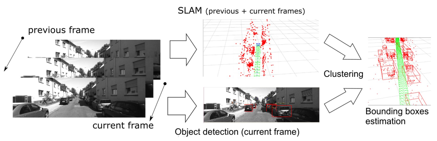
A diagram illustrating the general process flow in a SLAM system, highlighting sensor data input, tracking, mapping, and loop closure. Both filtering and smoothing are backend choices for the estimation part. Image Source: MDPI Sensors, SLAM-OR.

Data Usage and Estimation Focus

Filtering SLAM primarily uses current measurements and motion data to update the current state. Past information is summarized within the current state's probability distribution. Its focus is on "where am I now?" and "what does the immediate map look like?"

Smoothing SLAM, conversely, uses all or a large batch of past measurements. It aims to refine the entire history of poses and the complete map. Its focus is on "what was my entire path, and what is the globally consistent map?"

Accuracy and Consistency

Filtering SLAM can be prone to drift over long trajectories. Linearization errors (in EKF) and the Markov assumption (that the past is fully captured by the current state) can lead to inconsistencies. While effective for short-term localization, cumulative errors can degrade map quality and pose estimates over time. As noted in studies like the comparison by Herranz et al. (2014) for range-only SLAM, filtering approaches are generally less accurate than smoothing for the full trajectory.

Smoothing SLAM generally achieves higher accuracy and global consistency. By optimizing over the entire set of measurements, it can effectively incorporate loop closures (recognizing previously visited locations) to correct past estimates and reduce accumulated drift. This ability to re-linearize and re-evaluate past states leads to more robust and precise maps, especially in large-scale environments. Kaess et al. (2012) highlight how smoothing can provide globally optimal solutions.

Computational Complexity and Real-Time Capability

Filtering SLAM typically has a lower computational cost per time step because it only updates the current state. This makes it well-suited for real-time applications on resource-constrained platforms. However, for some filter types like EKF-SLAM, the computational complexity can increase, potentially quadratically, with the number of landmarks in the map if a dense covariance matrix is maintained.

Smoothing SLAM has historically been more computationally intensive, as optimizing a large graph of all past poses and measurements can be demanding. However, advancements like incremental smoothing (e.g., iSAM, iSAM2) and the exploitation of sparsity in the underlying mathematical problem (the information matrix in graph SLAM is often sparse) have significantly improved efficiency, enabling near real-time performance in many cases. Nevertheless, smoothing generally requires more memory and processing power than filtering. Strasdat et al. (2012) discuss these computational trade-offs, particularly in visual SLAM.

Robustness to Noise and Nonlinearities

Filtering SLAM, especially EKF-based methods, relies on assumptions of Gaussian noise and uses linearization for non-linear system models. These approximations can make filters fragile in highly non-linear environments or in the presence of non-Gaussian noise and outliers. Once linearization choices are made, they are typically not revisited, potentially leading to suboptimal solutions.

Smoothing SLAM is generally more robust to non-linearities and can better handle various noise models. Graph-based optimization allows for iterative refinement and re-linearization around better estimates. Furthermore, robust cost functions (e.g., Huber, Tukey) can be incorporated into the optimization framework to mitigate the influence of outliers in measurements.

A Visual Comparison of SLAM Algorithm Attributes

The radar chart below offers a visual summary of how filtering and smoothing SLAM algorithms compare across several key performance and characteristic attributes. This is a qualitative comparison based on typical implementations and general consensus in the field.

In this chart, higher values are generally better, except for 'Computational Cost' and 'Memory Usage' where lower values indicate better performance. Filtering SLAM excels in real-time capability and has lower computational costs and memory usage. Smoothing SLAM, on the other hand, offers superior overall accuracy, global consistency, and robustness to non-linearities.

Core Concepts Visualized: Filtering vs. Smoothing Mindmap

To further clarify the distinct characteristics and relationships, the following mindmap illustrates the core tenets of filtering and smoothing SLAM approaches.

mindmap root["SLAM Estimation Approaches"] id1["Filtering SLAM"] id1a["Recursive State Estimation"] id1b["Online / Real-time"] id1c["Focus: Current State"] id1d["Examples: EKF, UKF, Particle Filters"] id1e["Pros:
Lower computational cost per step
Good for immediate needs"] id1f["Cons:
Prone to drift
Linearization errors
Less globally consistent"] id2["Smoothing SLAM"] id2a["Batch or Incremental Optimization"] id2b["Offline / Less Frequent (or Incremental)"] id2c["Focus: Entire Trajectory & Map"] id2d["Examples: GraphSLAM, SAM, Bundle Adjustment"] id2e["Pros:
Higher accuracy
Global consistency
Robust to non-linearities
Effective loop closure"] id2f["Cons:
Higher computational cost (historically)
Higher memory usage"]

This mindmap provides a hierarchical view of the two main SLAM paradigms, branching out into their methodologies, operational characteristics, common examples, and their respective advantages and disadvantages.

Summary Table: Filtering vs. Smoothing SLAM

The following table provides a concise side-by-side comparison of key features:

Feature	Filtering SLAM	Smoothing SLAM
Principle	Recursive state estimation (e.g., Kalman filter, particle filter)	Batch or incremental optimization over entire trajectory (e.g., graph-based, MAP estimation)
Data Usage	Primarily current measurements; past data summarized or discarded	All or a large batch of past measurements retained and used
Estimation Focus	Estimates current robot pose and map features	Estimates entire robot trajectory and full map simultaneously
Operation Mode	Typically online, real-time	Typically offline or less frequent optimization; incremental methods improving real-time capability
Accuracy	Good for short-term; can suffer from drift and inconsistency over long trajectories	Generally higher accuracy and global consistency, especially with loop closures
Computational Complexity	Lower per step; can scale with map size (e.g., EKF covariance)	Historically higher, but improved with sparse methods and incremental techniques
Memory Usage	Lower, as it doesn't store all past data explicitly	Higher, as it often retains the entire graph of poses and measurements
Robustness to Non-linearities/Outliers	Can be sensitive due to linearization (EKF) and Gaussian assumptions	More robust; can handle non-linearities better through iteration and use robust cost functions
Examples	EKF-SLAM, UKF-SLAM, Particle Filter SLAM (e.g., FastSLAM)	GraphSLAM, SAM (Smoothing and Mapping), Bundle Adjustment, iSAM

Exploring Estimation in Time Series: Filtering, Smoothing, and Prediction

The concepts of filtering and smoothing are not unique to SLAM but are fundamental in time series analysis and state estimation. The following video provides a general introduction to these concepts, which helps in understanding their application within the SLAM context. While the video discusses Bayesian estimation broadly, the principles of using past, present, or future data to refine estimates are directly relevant.

In this video, "3.1 Filtering, smoothing and prediction," the speaker introduces three basic problems related to Bayesian estimation for time series. Filtering involves estimating the current state given all measurements up to the current time. This aligns with how filtering SLAM operates, providing an online estimate. Smoothing involves estimating a state at some point in the past, given all measurements up to the current time or even all measurements over the entire duration. This mirrors smoothing SLAM's approach of using the full dataset to refine past states and the overall trajectory. Prediction involves estimating a future state based on measurements up to the current time. While less central to the direct comparison of filtering vs. smoothing back-ends in SLAM, it's part of the broader state estimation toolkit often used in the prediction step of filters.

Understanding these general definitions aids in appreciating why smoothing approaches in SLAM can achieve higher accuracy by leveraging more information (including "future" data relative to a past state being estimated) compared to filtering, which is constrained to only past and current data for the current state estimate.

Practical Applications and Trends

Filtering-based SLAM remains relevant and widely used, particularly in applications with strict real-time constraints and limited computational resources. This includes many mobile robots, small aerial drones, and embedded systems where immediate pose updates are critical for navigation and control.

Smoothing-based SLAM has become increasingly dominant in applications demanding high precision and globally consistent maps. Autonomous vehicles, large-scale robotic exploration, augmented reality, and 3D reconstruction benefit significantly from the global optimization capabilities of smoothing. The trend in the SLAM community has leaned towards graph-based smoothing methods, especially with the development of efficient incremental solvers.

Hybrid approaches are also emerging, attempting to combine the strengths of both. For instance, a system might use filtering for fast, real-time state propagation and local map updates, while periodically performing smoothing or bundle adjustment over a sliding window of recent poses or the entire accumulated graph to maintain global consistency and refine the map. A technical report from EECS Berkeley (2021) discusses the "rapprochement" or convergence of these approaches, especially in visual-inertial SLAM.

Frequently Asked Questions (FAQ)

What is the fundamental difference between filtering and smoothing in SLAM?

The fundamental difference lies in how they use data to estimate the robot's state and map. Filtering algorithms process data sequentially and estimate only the current state, marginalizing out past states. They are typically online and computationally lighter per step. Smoothing algorithms, on the other hand, consider all (or a large window of) available data to jointly optimize the entire trajectory and map, leading to more globally consistent results but usually at a higher computational cost and often performed offline or in larger batches.

When should I choose filtering SLAM over smoothing SLAM?

Choose filtering SLAM when:

Real-time performance is critical and updates are needed at high frequency.
Computational resources (CPU, memory) are limited, such as on embedded systems or small robots.
The application primarily needs the current robot pose and local map, and minor global inconsistencies are acceptable or can be handled by other means.
Operating over shorter trajectories where drift accumulation is less problematic.

Are smoothing SLAM methods always more accurate than filtering methods?

Generally, smoothing SLAM methods offer higher global accuracy and consistency because they optimize over a larger set of data, allowing them to correct past errors and effectively utilize information like loop closures. However, "accuracy" can be context-dependent. For immediate, short-term localization, a well-tuned filter might perform adequately. Filtering methods can suffer from unrecoverable errors due to early incorrect linearizations or data associations, whereas smoothing methods can often mitigate these issues by re-evaluating past states during global optimization.

Can filtering and smoothing techniques be combined in SLAM?

Yes, hybrid approaches that combine filtering and smoothing are increasingly common. For example, a system might use a filter for high-frequency state estimation (odometry) and local mapping, while a smoothing component runs periodically or in a separate thread to perform global optimization, refine the map, and correct for drift. Sliding-window bundle adjustment is a form of smoothing applied to a recent window of poses, offering a compromise between full smoothing and pure filtering. Kaess et al. (2012) proposed methods for concurrent filtering and smoothing.

References

Last updated May 19, 2025