Comprehensive Report on Time Complexity and Space Complexity

Understanding the Efficiency and Resource Utilization of Algorithms

Key Takeaways

Time complexity evaluates how an algorithm's running time increases with input size, using Big O notation.
Space complexity assesses the memory usage of an algorithm relative to its input size, also expressed in Big O terms.
Optimizing both time and space complexities is crucial for developing efficient and scalable algorithms.

Introduction

In the realm of computer science, the efficiency of algorithms is paramount. Two fundamental metrics used to evaluate this efficiency are time complexity and space complexity. These metrics help developers and researchers understand how algorithms perform as the size of their input grows, guiding the selection and optimization of algorithms for various applications. This report delves into the definitions, classifications, analysis techniques, and practical considerations of time and space complexities, providing a comprehensive overview essential for anyone involved in algorithm design and optimization.

Time Complexity

Definition

Time complexity measures the amount of computational time an algorithm takes to process an input of size n. It quantifies the efficiency of an algorithm by expressing its running time as a function of the input size, typically using Big O notation. Big O provides an upper bound on the growth rate of the algorithm's runtime, offering insight into its performance in the worst-case scenario.

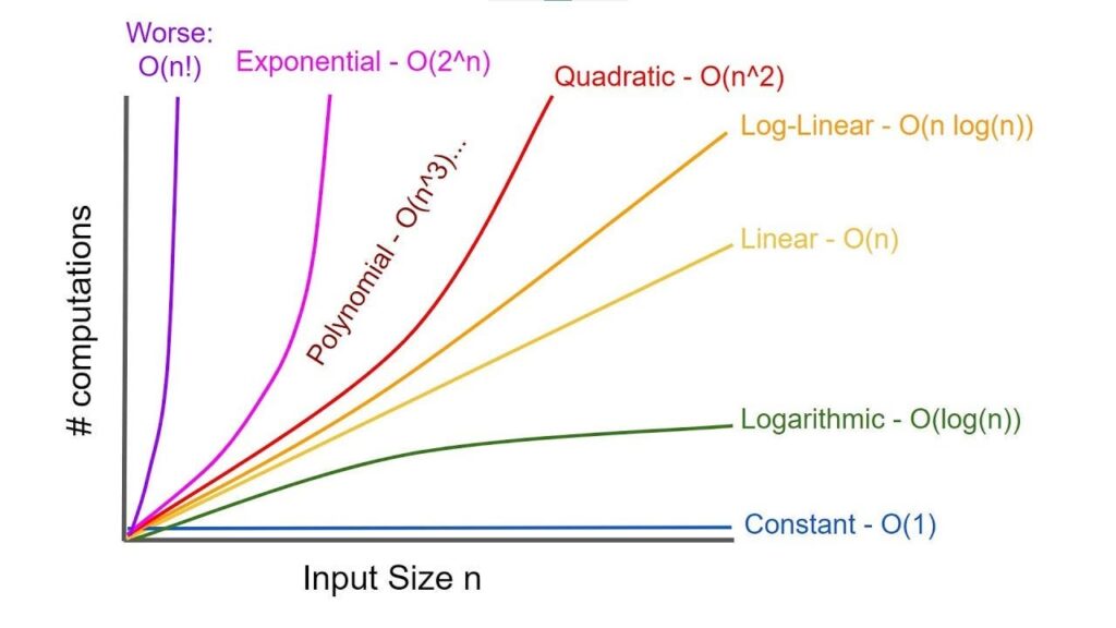
Key Time Complexity Categories

1. Constant Time – O(1)

An algorithm with constant time complexity performs its operations in a fixed amount of time, regardless of the input size. This efficiency is ideal for scenarios where rapid access or retrieval is essential.

Example: Accessing an element in an array by its index.

2. Logarithmic Time – O(log n)

Logarithmic time complexity indicates that the running time grows proportionally to the logarithm of the input size. Algorithms with this complexity are highly efficient for large inputs, as they reduce the problem size exponentially with each step.

Example: Binary search algorithm operating on a sorted array.

3. Linear Time – O(n)

Linear time complexity signifies that the running time increases directly in proportion to the input size. While not as efficient as logarithmic or constant time complexities, linear time algorithms are still practical for many applications.

Example: Iterating through each element in an array once.

4. Linearithmic Time – O(n log n)

Combining linear and logarithmic factors, linearithmic time complexity is common in highly efficient sorting algorithms. These algorithms scale well with input size, making them suitable for large datasets.

Example: Merge sort and quicksort algorithms.

5. Quadratic Time – O(n²)

Quadratic time complexity indicates that the running time grows proportionally to the square of the input size. This often results from algorithms with nested iterations over the same dataset, leading to significant performance degradation with larger inputs.

Example: Bubble sort and selection sort algorithms.

Analysis Techniques

Analyzing time complexity involves identifying the most significant operations that impact running time and expressing their frequency relative to input size. Common techniques include:

Loop Analysis: Evaluating the number of iterations in loops, especially nested loops, to determine their impact on time complexity.
Recurrence Relations: Used for recursive algorithms to express the running time in terms of input size and the number of recursive calls.
Best-case, Worst-case, and Average-case Analysis: Assessing how the algorithm performs under different input conditions.

Space Complexity

Definition

Space complexity measures the total memory an algorithm requires relative to the input size n. This includes the memory needed for input data, auxiliary data structures, and any additional space used during the algorithm's execution. Like time complexity, space complexity is expressed using Big O notation, providing a formal way to compare the memory efficiency of different algorithms.

Key Space Complexity Categories

1. Constant Space – O(1)

An algorithm with constant space complexity uses a fixed amount of memory regardless of the input size. This is the most memory-efficient category and is highly desirable in memory-constrained environments.

Example: Performing simple arithmetic operations without additional data structures.

2. Logarithmic Space – O(log n)

Logarithmic space complexity implies that the memory usage grows proportionally to the logarithm of the input size. This is typically seen in recursive algorithms that split the problem size by a constant factor at each step.

Example: Recursive implementations of binary search.

3. Linear Space – O(n)

Linear space complexity indicates that the memory usage increases linearly with the input size. This is common in algorithms that require additional storage proportional to the input, such as creating auxiliary arrays or lists.

Example: Creating an array to store input elements for a merge sort algorithm.

4. Quadratic Space – O(n²)

Quadratic space complexity denotes that the memory usage grows proportionally to the square of the input size. This typically arises in algorithms that use two-dimensional data structures or involve nested data processing.

Example: Using a two-dimensional array to represent a graph or adjacency matrix.

Analysis Techniques

Analyzing space complexity involves accounting for all memory allocations made by an algorithm relative to input size. Key methods include:

Counting Variable Allocations: Identifying all variables and data structures used by the algorithm and determining how their memory usage scales with input size.
Recursive Calls: Evaluating the additional memory consumed by the call stack during recursive executions.

Comparative Analysis of Time and Space Complexities

Time and space complexities often present a trade-off scenario where optimizing one can lead to increased usage of the other. Understanding and balancing these complexities is essential for designing efficient algorithms tailored to specific application needs. The following table illustrates common complexities with their descriptions and examples:

Complexity	Description	Example
O(1)	Constant time or space. Execution time or memory usage does not change with input size.	Accessing an array element by index.
O(log n)	Logarithmic time or space. Grows proportionally to the logarithm of the input size.	Binary search algorithm.
O(n)	Linear time or space. Grows directly with the input size.	Iterating through a list once.
O(n log n)	Linearithmic time. Combination of linear and logarithmic growth rates.	Merge sort algorithm.
O(n²)	Quadratic time or space. Grows proportionally to the square of the input size.	Bubble sort algorithm.

Practical Considerations

Trade-offs Between Time and Space

Often, enhancing an algorithm’s time efficiency results in increased space usage and vice versa. For instance, utilizing additional memory to store intermediate results can reduce the number of computations required, thereby speeding up the algorithm. Conversely, minimizing memory usage might necessitate performing more calculations, potentially slowing down the process. Balancing these trade-offs is crucial, especially in environments with limited resources.

Worst-case vs. Average-case Analysis

Time and space complexities can be analyzed under different scenarios:

Worst-case: Evaluates the maximum resources an algorithm might require, providing guarantees on its performance.
Average-case: Considers the expected resources needed over a range of possible inputs, offering a more realistic performance assessment.

The choice between worst-case and average-case analysis depends on the application context. For instance, real-time systems may prioritize worst-case guarantees to ensure consistent performance.

Hardware Constraints

The underlying hardware can influence the significance of time and space complexities. In systems with limited memory, algorithms with lower space complexities are preferred to prevent excessive memory consumption. Conversely, in environments where speed is critical, algorithms with lower time complexities may be prioritized, even if they require more memory.

Scalability

As applications handle increasingly large datasets, the scalability of algorithms becomes paramount. Efficient time and space complexities ensure that algorithms remain performant and resource-efficient as input sizes grow, making them suitable for large-scale data processing and high-performance computing scenarios.

Methods for Optimizing Algorithms

Algorithm Design Techniques

Various design techniques can help optimize time and space complexities:

Divide and Conquer: Breaking down a problem into smaller subproblems, solving them independently, and combining their solutions can lead to efficient algorithms, often with linearithmic time complexities.
Dynamic Programming: Storing the results of subproblems to avoid redundant computations, thereby optimizing time at the expense of additional memory usage.
Greedy Algorithms: Making the locally optimal choice at each step with the hope of finding the global optimum, typically leading to linear or linearithmic time complexities.
Memoization: Caching the results of expensive function calls to improve performance, similar to dynamic programming.

Data Structures

Selecting appropriate data structures can significantly impact both time and space complexities. Efficient data structures like hash tables, balanced trees, and heaps can optimize performance for various operations, such as search, insertion, and deletion.

Case Studies and Examples

Sorting Algorithms

Sorting algorithms provide clear examples of varying time and space complexities:

Bubble Sort: Has a time complexity of O(n²) and space complexity of O(1). It is simple but inefficient for large datasets.
Merge Sort: Exhibits a time complexity of O(n log n) and space complexity of O(n). It is efficient and stable, making it suitable for large inputs.
Quick Sort: Typically has a time complexity of O(n log n) on average but can degrade to O(n²) in the worst case. Its space complexity is O(log n) due to recursive calls.

Search Algorithms

Searching algorithms also demonstrate differences in complexities:

Linear Search: Features a time complexity of O(n) and space complexity of O(1), making it simple but less efficient for large, unsorted datasets.
Binary Search: Offers a time complexity of O(log n) and space complexity of O(1) for iterative implementations, but O(log n) space complexity for recursive implementations. It requires the dataset to be sorted.

Implications in Real-world Applications

Database Management Systems

Efficient query processing and indexing in databases rely heavily on algorithms with optimal time and space complexities. For instance, B-trees offer logarithmic time complexities for insertions, deletions, and searches, making them ideal for indexing large databases.

Machine Learning and Data Science

Machine learning algorithms must handle vast amounts of data efficiently. Optimizing time and space complexities ensures that models can be trained and deployed effectively on large datasets without prohibitive resource consumption.

Web Development

In web development, backend algorithms must process client requests swiftly and manage server resources judiciously. Efficient algorithms contribute to faster response times and scalable web applications capable of handling high traffic volumes.

Conclusion

Time complexity and space complexity are indispensable metrics in the evaluation and optimization of algorithms. Understanding these complexities enables developers to design algorithms that are not only efficient in execution but also mindful of resource constraints. As the scale of applications continues to grow, the importance of algorithmic efficiency becomes increasingly critical, driving advancements in computer science and technology. Mastery of these concepts is essential for anyone aiming to develop high-performance, scalable, and resource-efficient software solutions.

References

Last updated February 15, 2025