Unlocking the Secrets of Time Series Analysis

Discover the underlying patterns, trends, and forecasting methods in sequential data

Key Highlights

Understanding Time Series: Learn how sequential data points unveil trends, seasonality, and random fluctuations.
Analytical Techniques: Explore decomposition, forecasting methods like ARIMA, and other models for reliable predictions.
Visualization & Examples: See diagrams, charts, and practical examples from finance, meteorology, and more.

Concept of Time Series Analysis

Time series analysis is a powerful statistical method used to evaluate data that has been measured, observed, or recorded at successive time intervals. It involves the examination of data points over time to uncover important patterns such as trends, seasonal variations, cyclical behaviors, and random fluctuations. By breaking down data into these components, analysts can identify underlying patterns, make data‑driven predictions, and develop models that forecast future outcomes.

The sequence of measurements is crucial because the temporal order offers insights into how variables evolve. This intrinsic characteristic of time series data differentiates it from cross-sectional data, which contains observations taken at a single point in time. The ability to predict based on historical data is what makes time series analysis invaluable in various fields, including finance, economics, meteorology, and even smart technology applications.

Fundamental Components of Time Series Data

1. Trend

The trend component displays the long-term progression of the data. Analysts identify whether the data shows an upward, downward, or constant trend over a long period. Trends might be linear or nonlinear, and their accurate identification is vital for understanding the overall direction of the data.

2. Seasonality

Seasonality refers to patterns that repeat at regular intervals due to recurring factors. Common examples include daily, monthly, or yearly cycles such as increased retail sales during holidays, or temperature variations with seasonal changes. Recognizing seasonality helps in differentiating periodic fluctuations from true long-term trends.

3. Cyclical Variations

Unlike regular seasonality, cyclical variations are long-term oscillations that occur as part of economic or business cycles. These cycles are irregular and may be influenced by factors like economic conditions, political changes, or unconventional market events.

4. Irregularity (Noise)

Irregular or random components represent unpredictable fluctuations in the data that cannot be attributed to trend, seasonality, or cycles. This randomness is often referred to as noise and includes anomalies due to unforeseen events.

Decomposing time series data into these fundamental components not only aids in understanding the historical patterns but also refines the accuracy of predictive models.

Methods and Techniques for Analyzing Time Series Data

A combination of statistical, mathematical, and graphical approaches are used in time series analysis to diagnose and predict behavior in sequential data. Various techniques include:

Data Collection and Preprocessing

Consistent data collection at regular intervals is the first step. Whether collecting data on daily stock prices, monthly sales numbers, or annual GDP values, maintaining consistency in measurements and intervals is essential. Preprocessing involves cleaning the data, managing missing values, and normalizing data where necessary.

Visualization Techniques

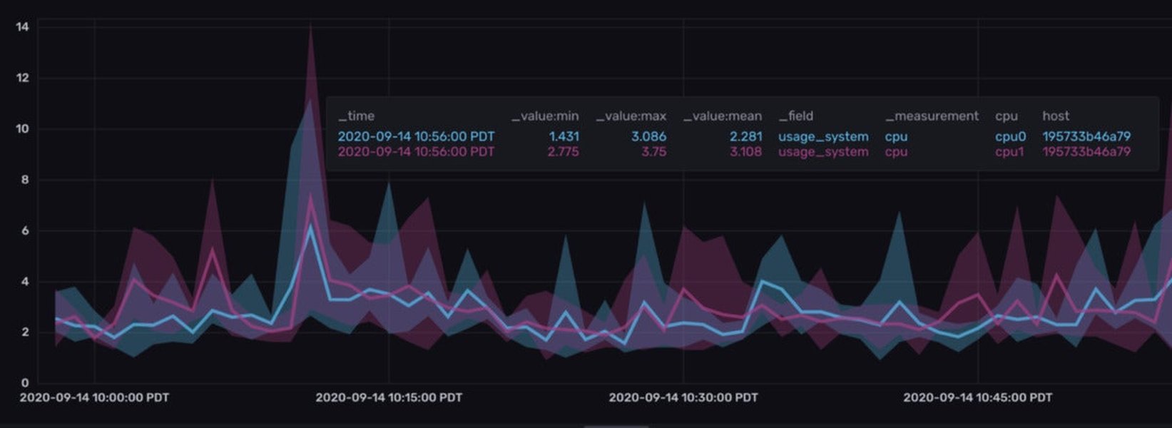
Graphical representations play a key role in time series analysis. They help visualize patterns, detect anomalies, and validate trends intuitively. Common visualization tools include:

Line Graphs: Display the continuous flow of data over time with time on the horizontal axis and the variable of interest on the vertical axis.
Seasonal Decomposition Plots: Separate the data into trend, seasonal, and residual components for comparative analysis.
Histograms and Autocorrelation Plots: Help in understanding the frequency distribution and relationships between lagged data points.

These visualizations not only facilitate pattern recognition but also assist in validating the outputs of statistical models.

Modeling and Forecasting

Time series analysis heavily relies on forecasting models that use historical data to predict future values. Techniques include:

Autoregressive (AR) Models: Forecast future values based solely on past values of the variable.
Moving Average (MA) Models: Utilize past forecast errors in a regression-like model.
ARIMA Models: Combine AR and MA models with differencing to address non-stationary data.
Exponential Smoothing (ES): Apply weighted averages of past observations where the weights decay exponentially.

Accurate modeling often involves checking for stationarity (ensuring statistical properties of the series are constant over time) and fine-tuning the parameters of the selected model to achieve robust predictions.

Visual Representations in Time Series Analysis

Diagrams and charts are critical for conveying insights derived from time series data. Below is a radar chart that combines various aspects of time series analysis based on opinionated analyses from diverse domains:

This radar chart juxtaposes the perceived strengths in different aspects of time series analysis across finance, meteorology, and sales forecasting. The insights from these datasets highlight varying levels of trend identification, seasonal variations, and the overall volume of data required for robust forecasting.

Detailed Examples and Diagrams

To provide a comprehensive understanding, the table below integrates various examples of time series analysis along with the related diagrams and key concepts.

Example	Description	Visualization
Stock Market Analysis	Evaluates daily stock prices to identify long-term trends, seasonal peaks, and random market fluctuations.	Line Graph, Seasonal Decomposition Plot
Sales Forecasting	Uses historical sales data to predict future product demand, identify seasonal patterns, and optimize inventory management.	Line Chart, Histogram, Forecasting Plot
Weather Forecasting	Analyzes temperature, precipitation, and wind speed data over time to predict future climate conditions and seasonal changes.	Time Series Plot, Autocorrelation Graph, Spectral Density Plot
Traffic Flow Analysis	Examines vehicle counts or sensor data to forecast traffic congestion and improve signal timings.	Line Graph, Decomposition Plot

In each case, visual diagrams such as time series plots and decomposition analyses are essential. They not only guide the detection of underlying trends but also validate the performance of forecasting models.

Exemplary Case Studies

1. Financial Markets

In the financial sector, time series analysis is primarily utilized to inspect historical price movements and forecast future trends. Analysts deploy models such as ARIMA and moving averages to anticipate price movements and identify market volatility. Visual charts such as line graphs help to illustrate these trends and seasonal peaks that might coincide with fiscal quarters or economic events.

2. Weather Forecasting

Meteorologists apply time series analysis to weather-related data to track daily temperatures, precipitation levels, and wind speeds. Seasonal components clearly appear in the data, enabling the prediction of weather patterns throughout the year. Decomposition plots make it simpler to separate the trend from irregular weather events, thereby enhancing the reliability of forecasts.

3. Sales and Demand Forecasting

Companies routinely use time series analysis to forecast sales and manage inventory levels. By identifying cyclic patterns and seasonal variations in consumer behavior, businesses can establish marketing strategies and manage supply chains more effectively. The combination of historical data and forecasting models like exponential smoothing allows businesses to mitigate risks associated with demand fluctuations.

4. Healthcare Monitoring

In healthcare, time series analysis helps monitor patient outcomes such as blood pressure and glucose levels over time. By continuously recording these metrics, clinicians can observe trends and spot sudden excursions from the norm, which may indicate health issues requiring immediate intervention.

Interactive FAQ Section

What is time series analysis?

Time series analysis is a statistical technique that analyzes data points collected or recorded at successive, evenly spaced time intervals. It involves decomposing the data into components such as trend, seasonality, cycles, and irregularity to understand underlying patterns and forecast future values.

Which statistical models are commonly used in time series forecasting?

Popular models include Autoregressive (AR), Moving Average (MA), ARIMA (Autoregressive Integrated Moving Average), and Exponential Smoothing. Each of these models captures different aspects of time-dependent data and is chosen based on the characteristics of the dataset and the forecasting objectives.

How do visualization techniques support time series analysis?

Visualization techniques such as line graphs, seasonal decomposition plots, and autocorrelation charts help in identifying long-term trends, periodic patterns, and irregular fluctuations in the data. These visual tools not only enhance the interpretability of complex datasets but also validate the results obtained from modeling.

Can time series analysis be applied to non-financial data?

Yes, time series analysis is widely applicable in numerous fields beyond finance. It is commonly used in meteorology for weather forecasting, in healthcare to monitor patient data, in sales for forecasting demand, and even in traffic management to optimize flow and reduce congestion.